Expected Running Times and Randomized Algorithms Instructor Neelima

Expected Running Times and Randomized Algorithms Instructor Neelima Gupta ngupta@cs. du. ac. in

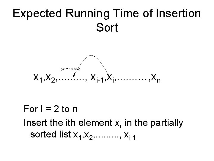
Expected Running Time of Insertion Sort (at rth position) x 1, x 2, . . , xi-1, xi, . . . . …, xn For I = 2 to n Insert the ith element xi in the partially sorted list x 1, x 2, . . , xi-1.

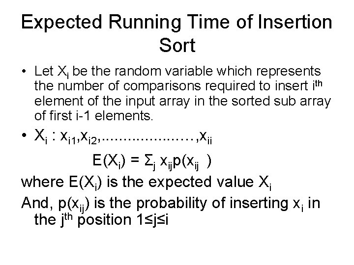
Expected Running Time of Insertion Sort • Let Xi be the random variable which represents the number of comparisons required to insert ith element of the input array in the sorted sub array of first i-1 elements. • Xi : xi 1, xi 2, . . . . …, xii E(Xi) = Σj xijp(xij ) where E(Xi) is the expected value Xi And, p(xij) is the probability of inserting xi in the jth position 1≤j≤i

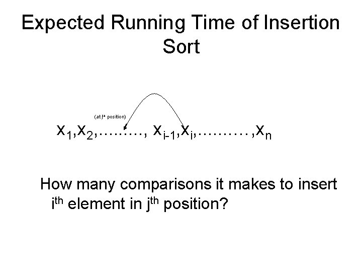
Expected Running Time of Insertion Sort (at jth position) x 1, x 2, . . , xi-1, xi, . . . . …, xn How many comparisons it makes to insert ith element in jth position?

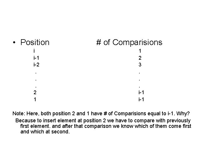
• Position i i-1 i-2. . . 2 1 # of Comparisions 1 2 3. . . i-1 Note: Here, both position 2 and 1 have # of Comparisions equal to i-1. Why? Because to insert element at position 2 we have to compare with previously first element. and after that comparison we know which of them come first and which at second.

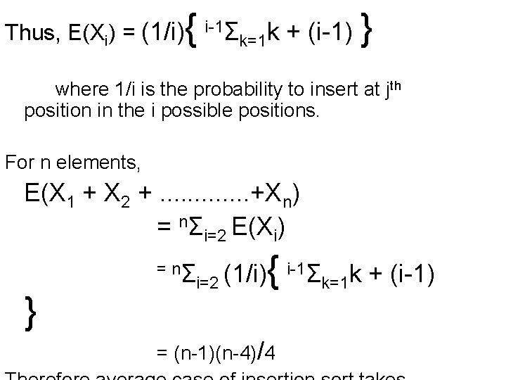
Thus, E(Xi) = (1/i) { i-1Σk=1 k + (i-1) } where 1/i is the probability to insert at jth position in the i possible positions. For n elements, E(X 1 + X 2 +. . . +Xn) = nΣi=2 E(Xi) = nΣ } i-1Σ (1/i) { i=2 k=1 k + (i-1) = (n-1)(n-4)/4

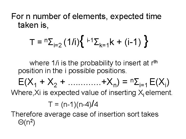
For n number of elements, expected time taken is, T = nΣi=2 (1/i) { i-1Σk=1 k + (i-1) } where 1/i is the probability to insert at rth position in the i possible positions. E(X 1 + X 2 +. . . +Xn) = nΣi=1 E(Xi) Where, Xi is expected value of inserting Xi element. T = (n-1)(n-4)/4 Therefore average case of insertion sort takes Θ(n 2)

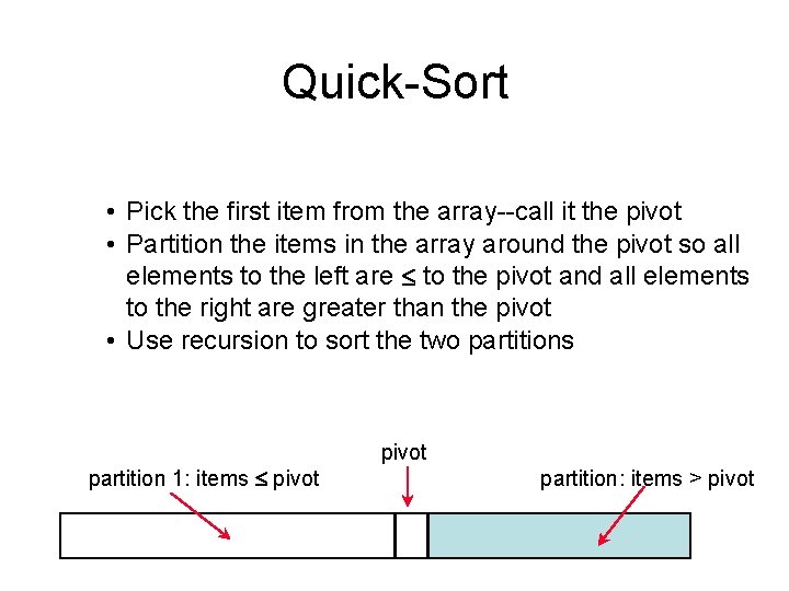
Quick-Sort • Pick the first item from the array--call it the pivot • Partition the items in the array around the pivot so all elements to the left are to the pivot and all elements to the right are greater than the pivot • Use recursion to sort the two partitions partition 1: items pivot partition: items > pivot

Quicksort: Expected number of comparisons • Partition may generate splits (0: n-1, 1: n-2, 2: n-3, … , n-2: 1, n-1: 0) each with probability 1/n • If T(n) is the expected running time,

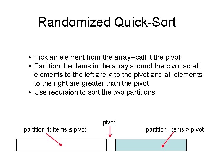
Randomized Quick-Sort • Pick an element from the array--call it the pivot • Partition the items in the array around the pivot so all elements to the left are to the pivot and all elements to the right are greater than the pivot • Use recursion to sort the two partitions partition 1: items pivot partition: items > pivot

Remarks • Not much different from the Q-sort except that earlier, the algorithm was deterministic and the bounds were probabilistic. • Here the algorithm is also randomized. We pick an element to be a pivot randomly. Notice that there isn’t any difference as to how does the algorithm behave there onwards? • In the earlier case, we can identify the worst case input. Here no input is worst

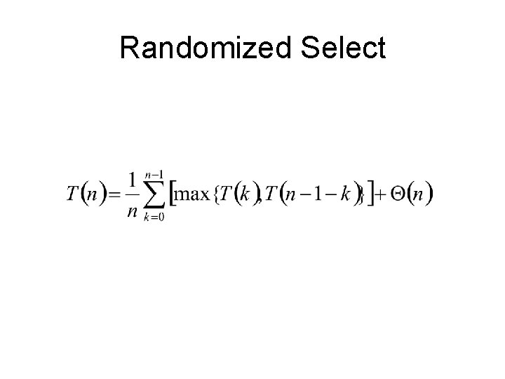
Randomized Select

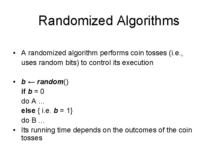
Randomized Algorithms • A randomized algorithm performs coin tosses (i. e. , uses random bits) to control its execution • b ← random() if b = 0 do A … else { i. e. b = 1} do B … • Its running time depends on the outcomes of the coin tosses

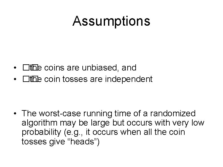
Assumptions • �� the coins are unbiased, and • �� the coin tosses are independent • The worst-case running time of a randomized algorithm may be large but occurs with very low probability (e. g. , it occurs when all the coin tosses give “heads”)

Monte Carlo Algorithms • Running times are guaranteed but the output may not be completely correct. • Probability of error is low.

Las Vegas Algorithms • Output is guaranteed to be correct. • Bounds on running times hold with high probability. • What type of algorithm is Randomized Qsort?

Why expected running times? • Markov’s inequality P( X > k E(X)) < 1/k i. e. the probability that the algorithm will take more than O(2 E(X)) time is less than 1/2. Or the probability that the algorithm will take more than O(10 E(X)) time is less than 1/10. This is the reason why Qsort does well in practice.

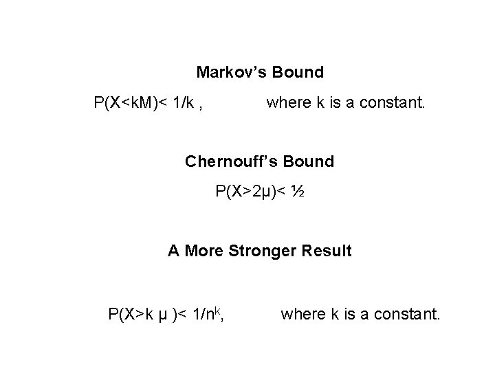
Markov’s Bound P(X<k. M)< 1/k , where k is a constant. Chernouff’s Bound P(X>2μ)< ½ A More Stronger Result P(X>k μ )< 1/nk, where k is a constant.

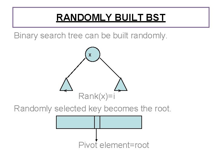
RANDOMLY BUILT BST Binary search tree can be built randomly. x < > Rank(x)=i Randomly selected key becomes the root. Pivot element=root

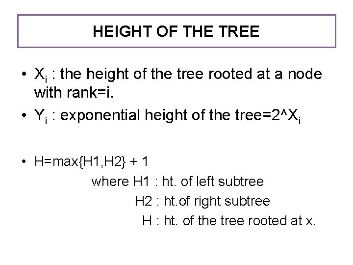
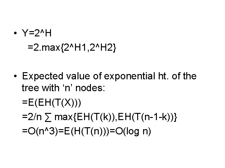
HEIGHT OF THE TREE • Xi : the height of the tree rooted at a node with rank=i. • Yi : exponential height of the tree=2^Xi • H=max{H 1, H 2} + 1 where H 1 : ht. of left subtree H 2 : ht. of right subtree H : ht. of the tree rooted at x.

• Y=2^H =2. max{2^H 1, 2^H 2} • Expected value of exponential ht. of the tree with ‘n’ nodes: =E(EH(T(X))) =2/n ∑ max{EH(T(k)), EH(T(n-1 -k))} =O(n^3)=E(H(T(n)))=O(log n)

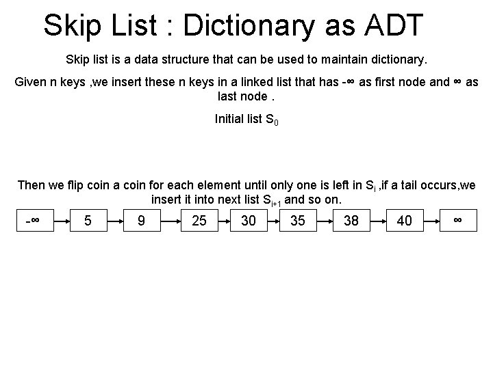
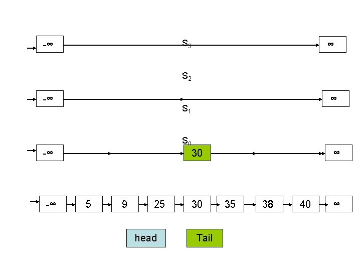
Skip List : Dictionary as ADT Skip list is a data structure that can be used to maintain dictionary. Given n keys , we insert these n keys in a linked list that has -∞ as first node and ∞ as last node. Initial list S 0 Then we flip coin a coin for each element until only one is left in Si , if a tail occurs, we insert it into next list Si+1 and so on. -∞ 5 9 25 30 35 38 40 ∞

S 3 -∞ ∞ S 2 -∞ ∞ S 1 S 0 -∞ -∞ 30 5 9 25 head 30 Tail ∞ 35 38 40 ∞

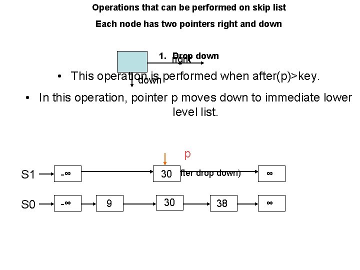
Operations that can be performed on skip list Each node has two pointers right and down 1. right Drop down • This operation is performed when after(p)>key. down • In this operation, pointer p moves down to immediate lower level list. p S 1 -∞ S 0 -∞ 9 30 (after drop down) ∞ 30 ∞ 38

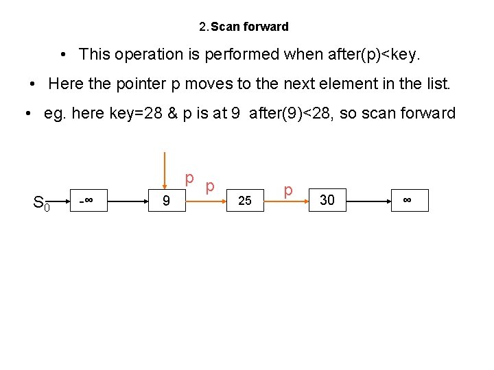
2. Scan forward • This operation is performed when after(p)<key. • Here the pointer p moves to the next element in the list. • eg. here key=28 & p is at 9 after(9)<28, so scan forward S 0 -∞ 9 p p 25 p 30 ∞

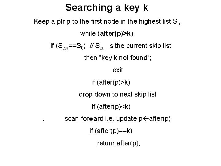
Searching a key k Keep a ptr p to the first node in the highest list Sh while (after(p)>k) if (Scur==S 0) // Scur is the current skip list then “key k not found”; exit if (after(p)>k) drop down to next skip list If (after(p)<k). scan forward i. e. update p after(p) if (after(p)==k) return after(p);

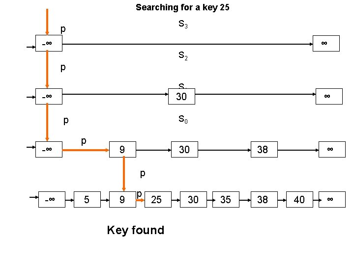
Searching for a key 25 S 3 p -∞ ∞ S 2 p S 1 -∞ 30 S 0 p -∞ ∞ p 9 30 38 ∞ p -∞ 5 9 p 25 Key found 30 35 38 40 ∞

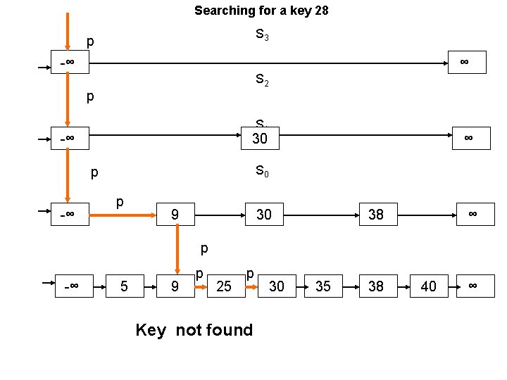
Searching for a key 28 S 3 p -∞ ∞ S 2 p S 1 -∞ 30 S 0 p -∞ ∞ p 9 30 38 ∞ p -∞ 5 9 p 25 p Key not found 30 35 38 40 ∞

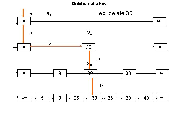
Deletion of a key eg. delete 30 S 3 p -∞ ∞ S 2 p p -∞ 30 S 1 ∞ p S 0 -∞ 9 30 38 ∞ p -∞ 5 9 25 30 35 38 40 ∞

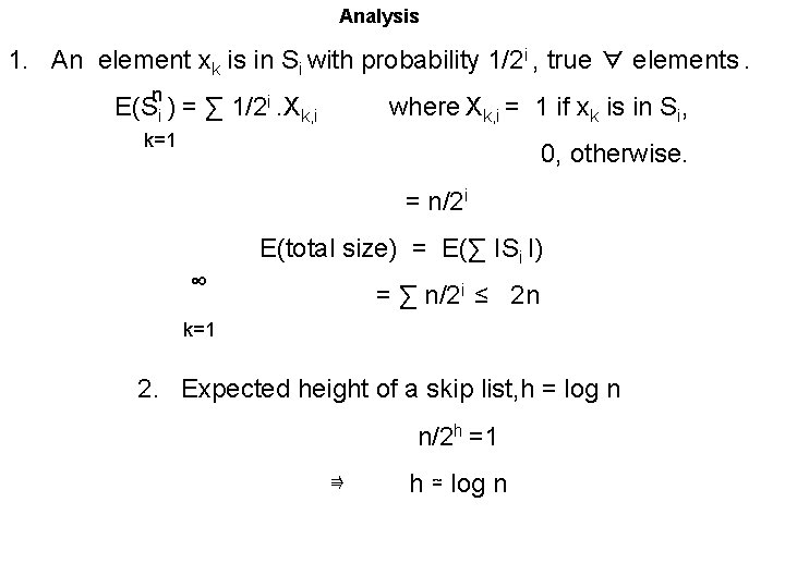
Analysis 1. An element xk is in Si with probability 1/2 i , true ∀ elements. n E(Si ) = ∑ 1/2 i. Xk, i where Xk, i = 1 if xk is in Si, k=1 0, otherwise. = n/2 i E(total size) = E(∑ ISi I) ∞ = ∑ n/2 i ≤ 2 n k=1 2. Expected height of a skip list, h = log n n/2 h =1 ⇛ h ≃ log n

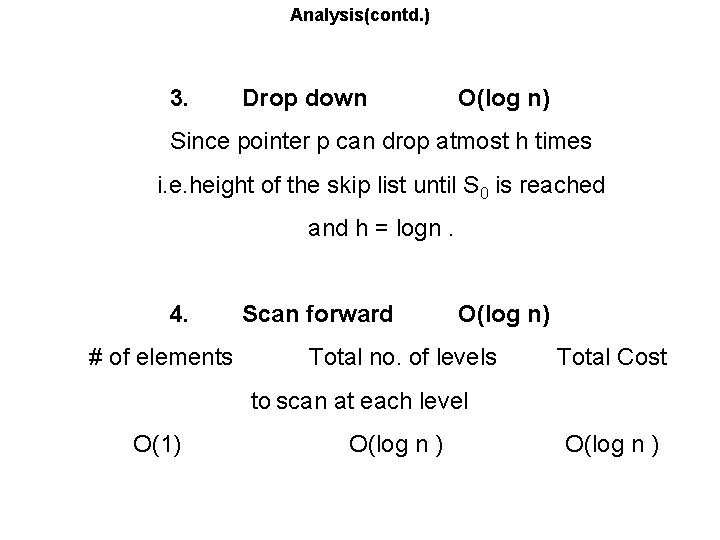
Analysis(contd. ) 3. Drop down O(log n) Since pointer p can drop atmost h times i. e. height of the skip list until S 0 is reached and h = logn. 4. # of elements Scan forward O(log n) Total no. of levels Total Cost to scan at each level O(1) O(log n )

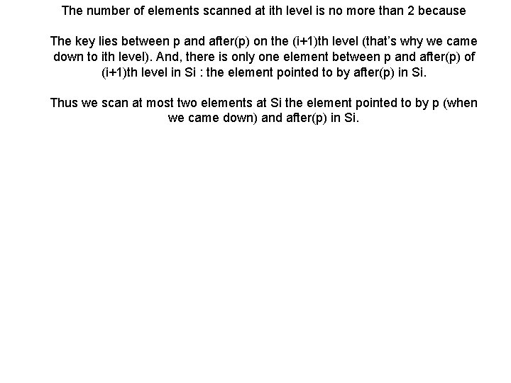
The number of elements scanned at ith level is no more than 2 because The key lies between p and after(p) on the (i+1)th level (that’s why we came down to ith level). And, there is only one element between p and after(p) of (i+1)th level in Si : the element pointed to by after(p) in Si. Thus we scan at most two elements at Si the element pointed to by p (when we came down) and after(p) in Si.

Hashing • Motivation: symbol tables – A compiler uses a symbol table to relate symbols to associated data • Symbols: variable names, procedure names, etc. • Associated data: memory location, call graph, etc. – For a symbol table (also called a dictionary), we care about search, insertion, and deletion – We typically don’t care about sorted order

Hash Tables • More formally: – Given a table T and a record x, with key (= symbol) and satellite data, we need to support: • Insert (T, x) • Delete (T, x) • Search(T, x) – We want these to be fast, but don’t care about sorting the records • The structure we will use is a hash table – Supports all the above in O(1) expected time!

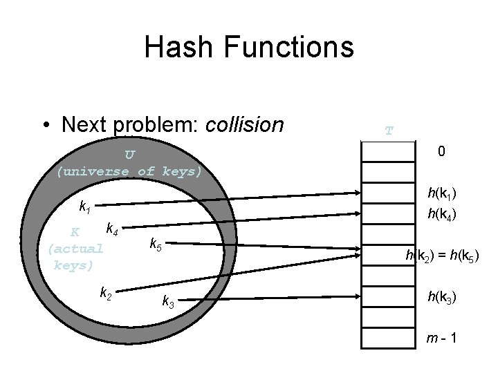
Hash Functions • Next problem: collision U (universe of keys) k 2 0 h(k 1) h(k 4) k 1 k 4 K (actual keys) T k 5 h(k 2) = h(k 5) k 3 h(k 3) m-1

Resolving Collisions • How can we solve the problem of collisions? • One of the solution is : chaining • Other solutions: open addressing

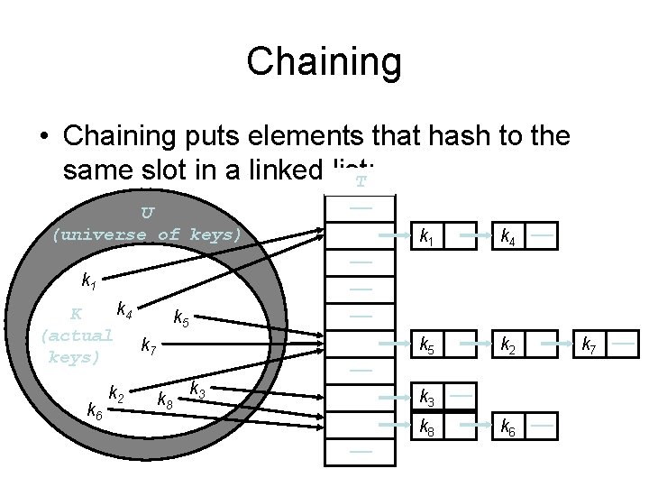
Chaining • Chaining puts elements that hash to the same slot in a linked list: T U (universe of keys) k 4 K k 5 (actual k 7 keys) k 6 k 8 k 1 k 4 —— k 5 k 2 —— —— —— k 1 k 2 —— k 3 —— k 8 —— k 6 —— k 7 ——

Chaining • How do we insert an element? U (universe of keys) k 4 K k 5 (actual k 7 keys) k 6 k 8 k 1 k 4 —— k 5 k 2 —— —— —— k 1 k 2 T —— k 3 —— k 8 —— k 6 —— k 7 ——

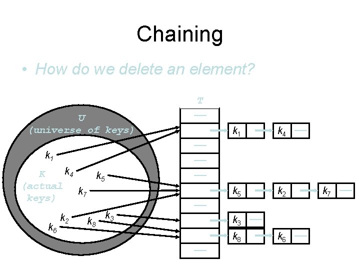
Chaining • How do we delete an element? U (universe of keys) k 4 K k 5 (actual k 7 keys) k 6 k 8 k 1 k 4 —— k 5 k 2 —— —— —— k 1 k 2 T —— k 3 —— k 8 —— k 6 —— k 7 ——

Chaining • How do we search for a element with a given key? T U (universe of keys) k 4 K k 5 (actual k 7 keys) k 6 k 8 k 1 k 4 —— k 5 k 2 —— —— —— k 1 k 2 —— k 3 —— k 8 —— k 6 —— k 7 ——

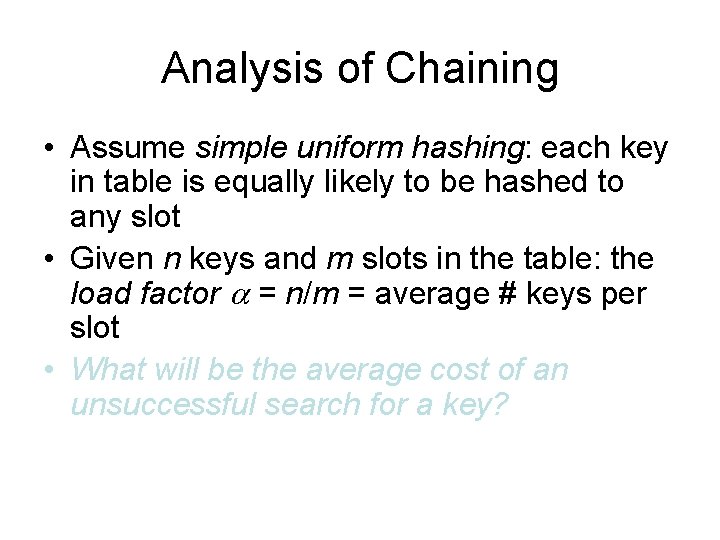
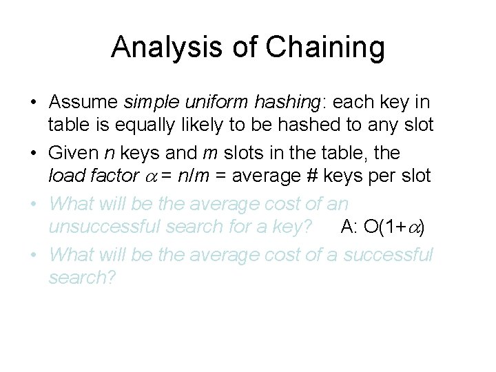
Analysis of Chaining • Assume simple uniform hashing: each key in table is equally likely to be hashed to any slot • Given n keys and m slots in the table: the load factor = n/m = average # keys per slot • What will be the average cost of an unsuccessful search for a key?

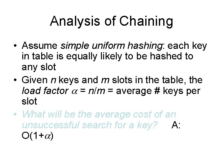
Analysis of Chaining • Assume simple uniform hashing: each key in table is equally likely to be hashed to any slot • Given n keys and m slots in the table, the load factor = n/m = average # keys per slot • What will be the average cost of an unsuccessful search for a key? A: O(1+ )

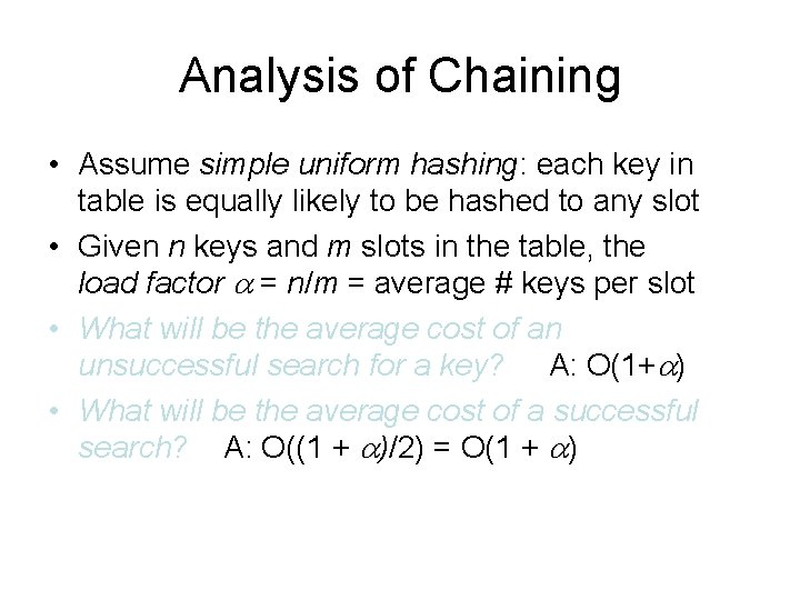
Analysis of Chaining • Assume simple uniform hashing: each key in table is equally likely to be hashed to any slot • Given n keys and m slots in the table, the load factor = n/m = average # keys per slot • What will be the average cost of an unsuccessful search for a key? A: O(1+ ) • What will be the average cost of a successful search?

Analysis of Chaining • Assume simple uniform hashing: each key in table is equally likely to be hashed to any slot • Given n keys and m slots in the table, the load factor = n/m = average # keys per slot • What will be the average cost of an unsuccessful search for a key? A: O(1+ ) • What will be the average cost of a successful search? A: O((1 + )/2) = O(1 + )

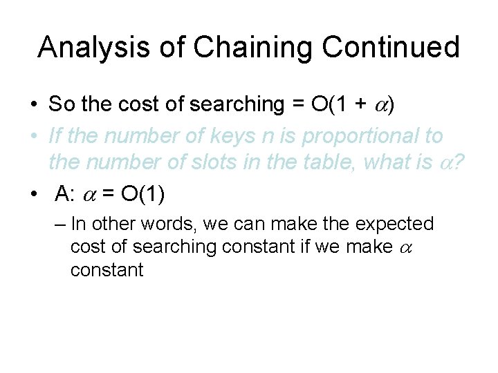
Analysis of Chaining Continued • So the cost of searching = O(1 + ) • If the number of keys n is proportional to the number of slots in the table, what is ? • A: = O(1) – In other words, we can make the expected cost of searching constant if we make constant

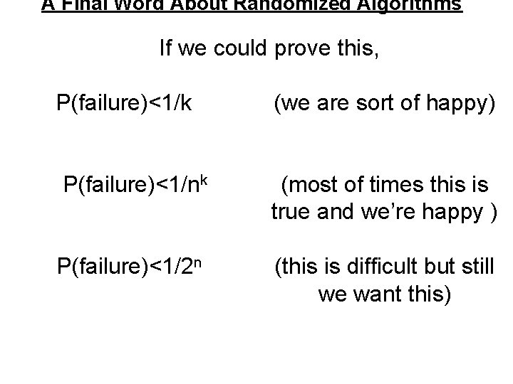
A Final Word About Randomized Algorithms If we could prove this, P(failure)<1/k (we are sort of happy) P(failure)<1/nk (most of times this is true and we’re happy ) P(failure)<1/2 n (this is difficult but still we want this)

Acknowledgements • Kunal Verma • Nidhi Aggarwal • And other students of MSc(CS) batch 2009.

END