Solving PDEs with CUDA Jonathan Cohen jocohennvidia com

Solving PDEs with CUDA Jonathan Cohen jocohen@nvidia. com NVIDIA Research

PDEs (Partial Differential Equations) Big topic Some common strategies Focus on one type of PDE in this talk Poisson Equation Linear equation => Linear solvers Parallel approaches for solving resulting linear systems © NVIDIA Corporation 2009

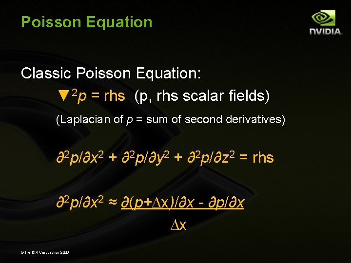
Poisson Equation Classic Poisson Equation: ▼ 2 p = rhs (p, rhs scalar fields) (Laplacian of p = sum of second derivatives) ∂2 p/∂x 2 + ∂2 p/∂y 2 + ∂2 p/∂z 2 = rhs ∂2 p/∂x 2 ≈ ∂(p+∆x)/∂x - ∂p/∂x ∆x © NVIDIA Corporation 2009

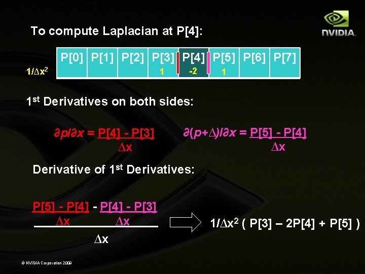
To compute Laplacian at P[4]: P[0] P[1] P[2] P[3] P[4] P[5] P[6] P[7] 1/∆x 2 1 -2 1 1 st Derivatives on both sides: ∂p/∂x = P[4] - P[3] ∆x ∂(p+∆)/∂x = P[5] - P[4] ∆x Derivative of 1 st Derivatives: P[5] - P[4] - P[3] ∆x ∆x ∆x © NVIDIA Corporation 2009 1/∆x 2 ( P[3] – 2 P[4] + P[5] )

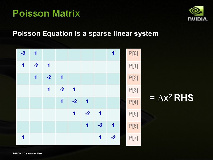
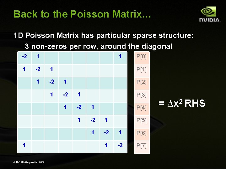
Poisson Matrix Poisson Equation is a sparse linear system -2 1 1 1 -2 P[1] 1 1 © NVIDIA Corporation 2009 P[0] P[2] 1 P[3] -2 1 1 -2 1 P[6] 1 -2 P[7] P[4] P[5] = ∆x 2 RHS

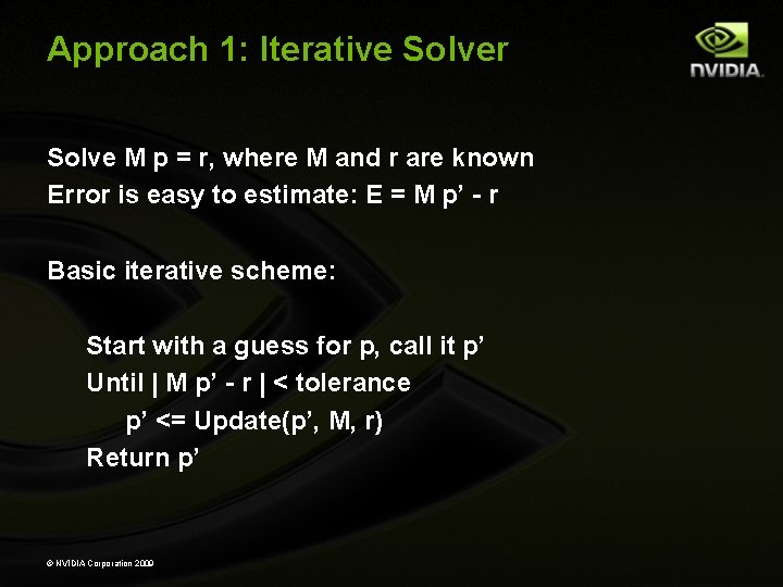
Approach 1: Iterative Solver Solve M p = r, where M and r are known Error is easy to estimate: E = M p’ - r Basic iterative scheme: Start with a guess for p, call it p’ Until | M p’ - r | < tolerance p’ <= Update(p’, M, r) Return p’ © NVIDIA Corporation 2009

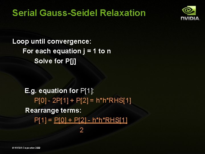
Serial Gauss-Seidel Relaxation Loop until convergence: For each equation j = 1 to n Solve for P[j] E. g. equation for P[1]: P[0] - 2 P[1] + P[2] = h*h*RHS[1] Rearrange terms: P[1] = P[0] + P[2] - h*h*RHS[1] 2 © NVIDIA Corporation 2009

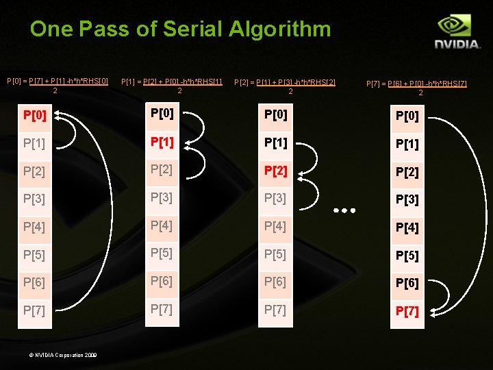
One Pass of Serial Algorithm P[0] = P[7] + P[1] -h*h*RHS[0] 2 P[1] = P[2] + P[0] -h*h*RHS[1] 2 P[2] = P[1] + P[3] -h*h*RHS[2] 2 P[7] = P[6] + P[0] -h*h*RHS[7] 2 P[0] P[1] P[2] P[3] P[4] P[5] P[6] P[7] © NVIDIA Corporation 2009

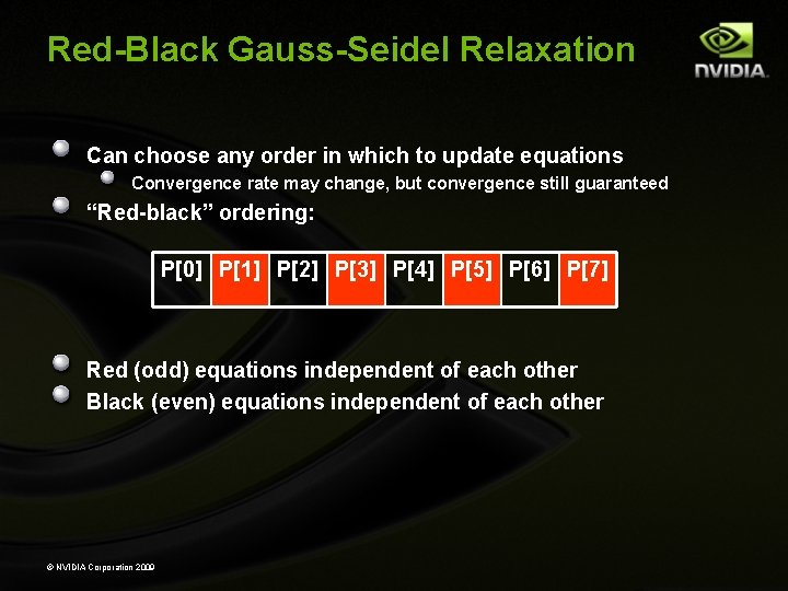
Red-Black Gauss-Seidel Relaxation Can choose any order in which to update equations Convergence rate may change, but convergence still guaranteed “Red-black” ordering: P[0] P[1] P[2] P[3] P[4] P[5] P[6] P[7] Red (odd) equations independent of each other Black (even) equations independent of each other © NVIDIA Corporation 2009

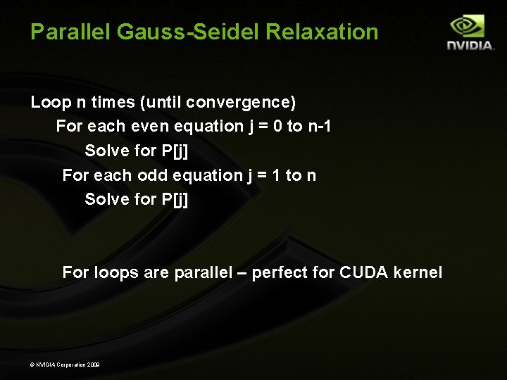
Parallel Gauss-Seidel Relaxation Loop n times (until convergence) For each even equation j = 0 to n-1 Solve for P[j] For each odd equation j = 1 to n Solve for P[j] For loops are parallel – perfect for CUDA kernel © NVIDIA Corporation 2009

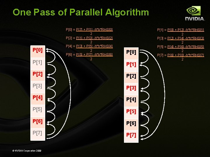
One Pass of Parallel Algorithm P[0] P[1] P[0] = P[7] + P[1] -h*h*RHS[0] 2 P[2] = P[1] + P[3] -h*h*RHS[2] 2 P[4] = P[3] + P[5] -h*h*RHS[4] 2 P[6] = P[5] + P[7] -h*h*RHS[6] 2 P[0] P[1] P[2] P[3] P[4] P[5] P[6] P[7] © NVIDIA Corporation 2009 P[1] = P[0] + P[2] -h*h*RHS[1] 2 P[3] = P[2] + P[4] -h*h*RHS[3] 2 P[5] = P[4] + P[6] -h*h*RHS[5] 2 P[7] = P[6] + P[0] -h*h*RHS[7] 2

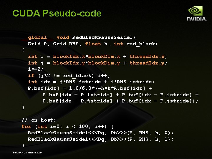
CUDA Pseudo-code __global__ void Red. Black. Gauss. Seidel( Grid P, Grid RHS, float h, int red_black) { int i = block. Idx. x*block. Dim. x + thread. Idx. x; int j = block. Idx. y*block. Dim. y + thread. Idx. y; i*=2; if (j%2 != red_black) i++; int idx = j*RHS. jstride + i*RHS. istride; P. buf[idx] = 1. 0/6. 0*(-h*h*R. buf[idx] + P. buf[idx + P. istride] + P. buf[idx – P. istride] + P. buf[idx + P. jstride] + P. buf[idx – P. jstride]); } // on host: for (int i=0; i < 100; i++) { Red. Black. Gauss. Seidel<<<Dg, Db>>>(P, RHS, h, 0); Red. Black. Gauss. Seidel<<<Dg, Db>>>(P, RHS, h, 1); } © NVIDIA Corporation 2009

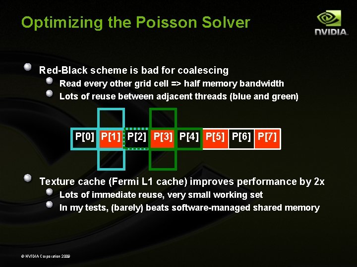
Optimizing the Poisson Solver Red-Black scheme is bad for coalescing Read every other grid cell => half memory bandwidth Lots of reuse between adjacent threads (blue and green) P[0] P[1] P[2] P[3] P[4] P[5] P[6] P[7] Texture cache (Fermi L 1 cache) improves performance by 2 x Lots of immediate reuse, very small working set In my tests, (barely) beats software-managed shared memory © NVIDIA Corporation 2009

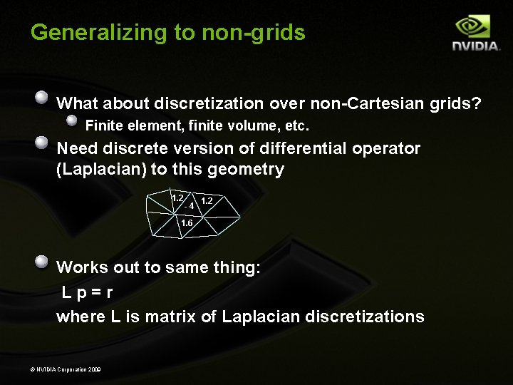
Generalizing to non-grids What about discretization over non-Cartesian grids? Finite element, finite volume, etc. Need discrete version of differential operator (Laplacian) to this geometry 1. 2 -4 1. 2 1. 6 Works out to same thing: Lp=r where L is matrix of Laplacian discretizations © NVIDIA Corporation 2009

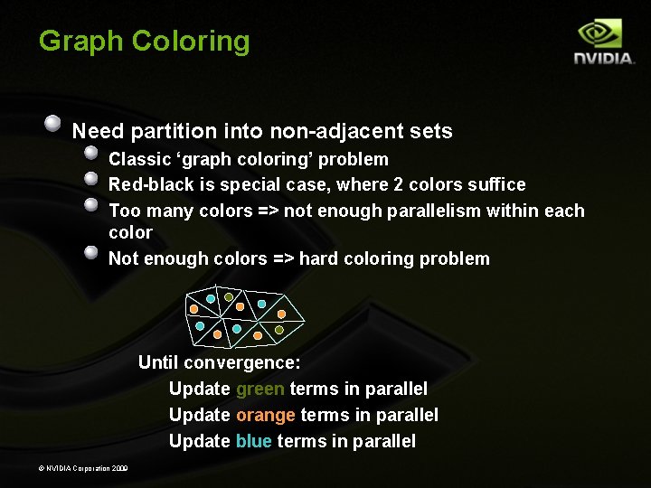
Graph Coloring Need partition into non-adjacent sets Classic ‘graph coloring’ problem Red-black is special case, where 2 colors suffice Too many colors => not enough parallelism within each color Not enough colors => hard coloring problem Until convergence: Update green terms in parallel Update orange terms in parallel Update blue terms in parallel © NVIDIA Corporation 2009

Back to the Poisson Matrix… 1 D Poisson Matrix has particular sparse structure: 3 non-zeros per row, around the diagonal -2 1 1 1 -2 P[1] 1 1 © NVIDIA Corporation 2009 P[0] P[2] 1 P[3] -2 1 1 -2 1 P[6] 1 -2 P[7] P[4] P[5] = ∆x 2 RHS

Approach 2: Direct Solver Solve the matrix equation directly Exploit sparsity pattern – all zeroes except diagonal, 1 above, 1 below = “tridiagonal” matrix Many applications for tridiagonal matrices Vertical diffusion (adjacent columns do not interact) ADI methods (e. g. separate 2 D blur x blur, y blur) Linear solvers (multigrid, preconditioners, etc. ) Typically many small tridiagonal systems => per-CTA algorithm © NVIDIA Corporation 2009

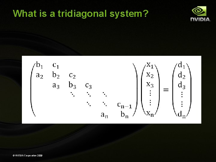
What is a tridiagonal system? © NVIDIA Corporation 2009

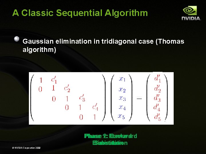
A Classic Sequential Algorithm Gaussian elimination in tridiagonal case (Thomas algorithm) Phase 1: 2: Forward Backward Elimination Substitution © NVIDIA Corporation 2009

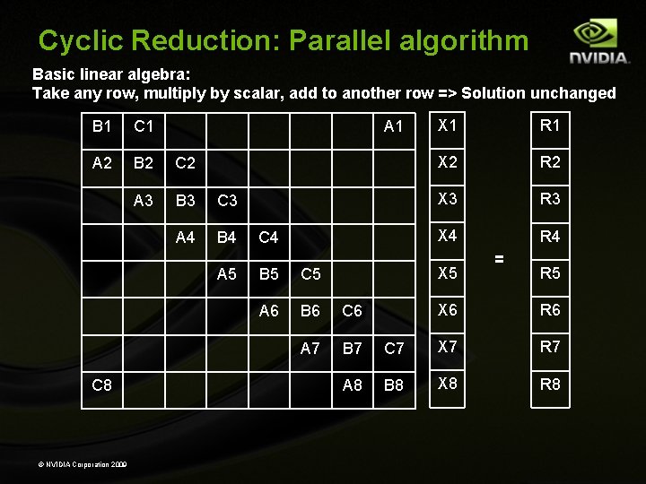
Cyclic Reduction: Parallel algorithm Basic linear algebra: Take any row, multiply by scalar, add to another row => Solution unchanged B 1 C 1 A 2 B 2 C 2 A 3 B 3 C 3 A 4 B 4 A 5 C 8 © NVIDIA Corporation 2009 C 4 X 1 R 1 X 2 R 2 X 3 R 3 X 4 R 4 X 5 B 5 C 5 A 6 B 6 C 6 A 7 B 7 A 8 = R 5 X 6 R 6 C 7 X 7 R 7 B 8 X 8 R 8

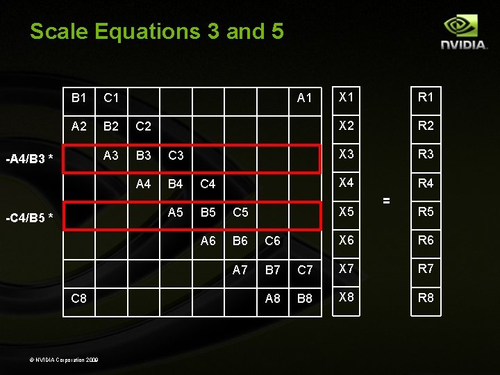
Scale Equations 3 and 5 B 1 C 1 A 2 B 2 C 2 A 3 B 3 C 3 A 4 B 4 -A 4/B 3 * A 1 A 5 -C 4/B 5 * C 8 © NVIDIA Corporation 2009 C 4 X 1 R 1 X 2 R 2 X 3 R 3 X 4 R 4 X 5 B 5 C 5 A 6 B 6 C 6 A 7 B 7 A 8 = R 5 X 6 R 6 C 7 X 7 R 7 B 8 X 8 R 8

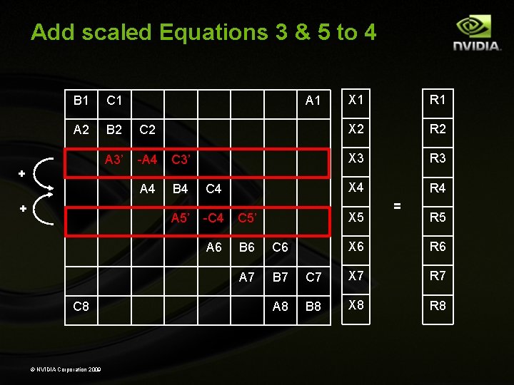
Add scaled Equations 3 & 5 to 4 B 1 C 1 A 2 B 2 C 2 A 3’ -A 4 C 3’ A 4 B 4 + + A 1 A 5’ C 8 © NVIDIA Corporation 2009 C 4 X 1 R 1 X 2 R 2 X 3 R 3 X 4 R 4 X 5 -C 4 C 5’ A 6 B 6 C 6 A 7 B 7 A 8 = R 5 X 6 R 6 C 7 X 7 R 7 B 8 X 8 R 8

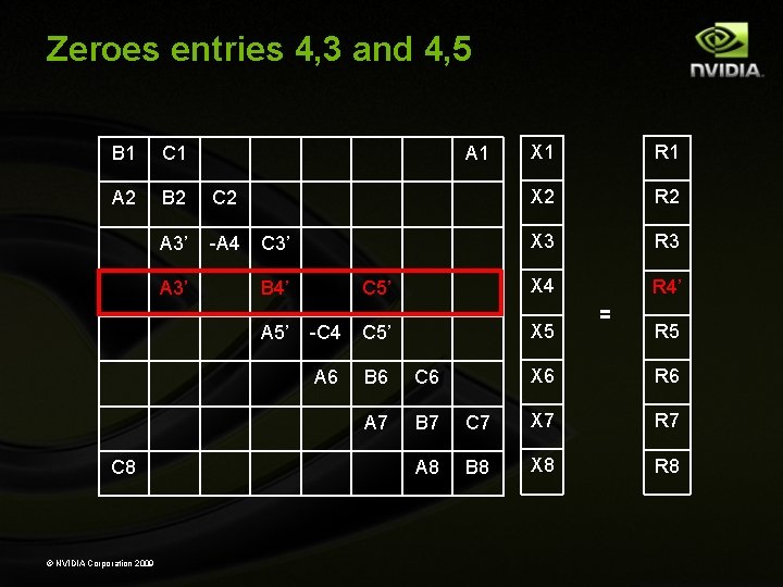
Zeroes entries 4, 3 and 4, 5 B 1 C 1 A 2 B 2 C 2 A 3’ -A 4 A 3’ A 1 C 3’ B 4’ A 5’ C 8 © NVIDIA Corporation 2009 C 5’ X 1 R 1 X 2 R 2 X 3 R 3 X 4 R 4’ X 5 -C 4 C 5’ A 6 B 6 C 6 A 7 B 7 A 8 = R 5 X 6 R 6 C 7 X 7 R 7 B 8 X 8 R 8

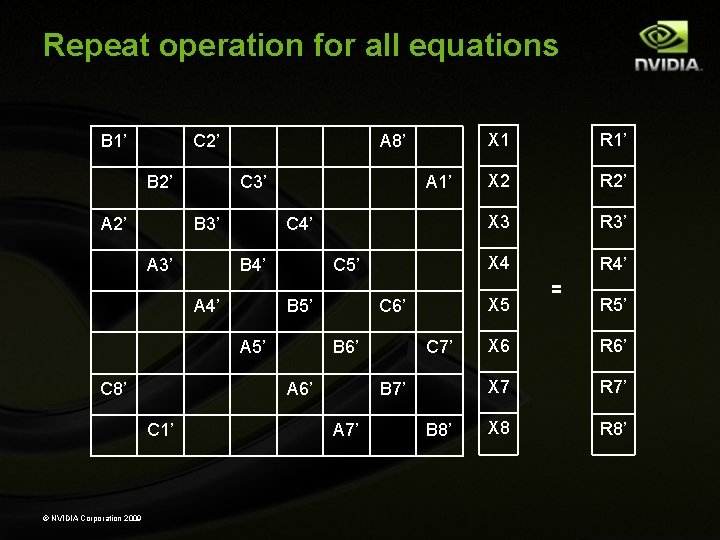
Repeat operation for all equations B 1’ C 2’ B 2’ A 8’ C 3’ B 3’ A 1’ C 4’ B 4’ A 4’ C 5’ B 5’ A 5’ C 8’ A 6’ C 1’ © NVIDIA Corporation 2009 C 7’ B 7’ A 7’ R 1’ X 2 R 2’ X 3 R 3’ X 4 R 4’ X 5 C 6’ B 6’ X 1 B 8’ = R 5’ X 6 R 6’ X 7 R 7’ X 8 R 8’

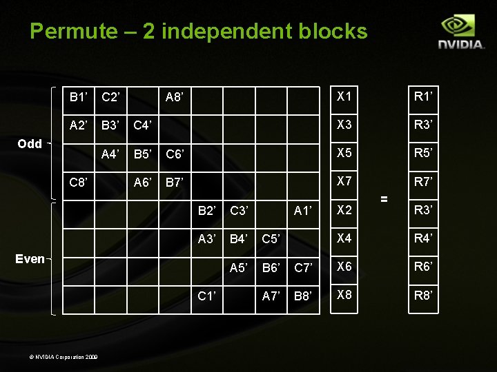
Permute – 2 independent blocks B 1’ C 2’ A 2’ B 3’ C 4’ A 4’ B 5’ A 6’ Odd C 8’ X 1 R 1’ X 3 R 3’ C 6’ X 5 R 5’ B 7’ X 7 R 7’ A 8’ B 2’ C 3’ A 3’ B 4’ C 5’ A 5’ B 6’ A 7’ Even C 1’ © NVIDIA Corporation 2009 A 1’ X 2 = R 3’ X 4 R 4’ C 7’ X 6 R 6’ B 8’ X 8 R 8’

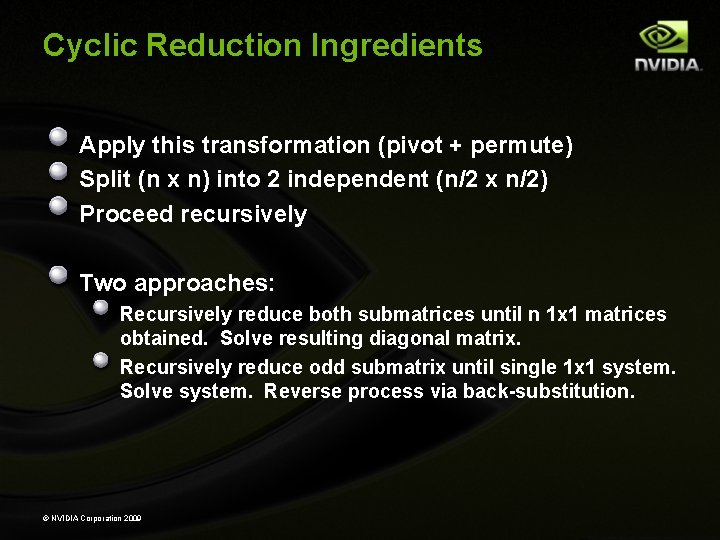
Cyclic Reduction Ingredients Apply this transformation (pivot + permute) Split (n x n) into 2 independent (n/2 x n/2) Proceed recursively Two approaches: Recursively reduce both submatrices until n 1 x 1 matrices obtained. Solve resulting diagonal matrix. Recursively reduce odd submatrix until single 1 x 1 system. Solve system. Reverse process via back-substitution. © NVIDIA Corporation 2009

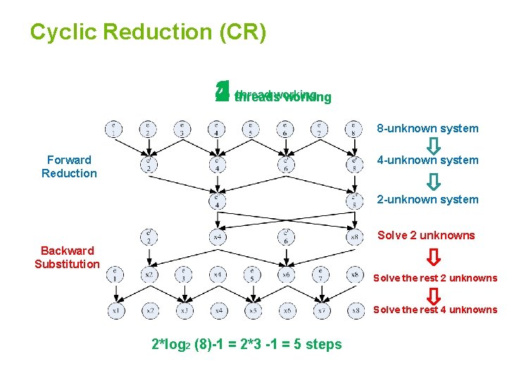
Cyclic Reduction (CR) 41 threads working 2 thread working 8 -unknown system Forward Reduction 4 -unknown system 2 -unknown system Solve 2 unknowns Backward Substitution Solve the rest 2 unknowns Solve the rest 4 unknowns 2*log 2 (8)-1 = 2*3 -1 = 5 steps © NVIDIA Corporation 2009

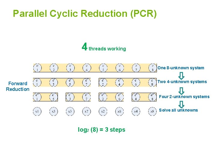
Parallel Cyclic Reduction (PCR) 4 threads working One 8 -unknown system Two 4 -unknown systems Forward Reduction Four 2 -unknown systems Solve all unknowns log 2 (8) = 3 steps © NVIDIA Corporation 2009

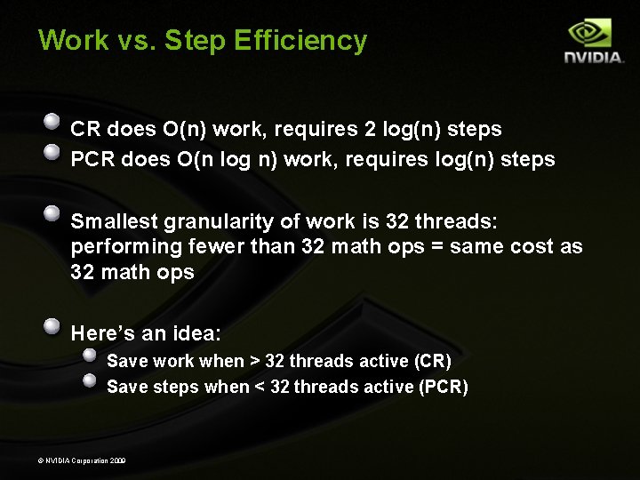
Work vs. Step Efficiency CR does O(n) work, requires 2 log(n) steps PCR does O(n log n) work, requires log(n) steps Smallest granularity of work is 32 threads: performing fewer than 32 math ops = same cost as 32 math ops Here’s an idea: Save work when > 32 threads active (CR) Save steps when < 32 threads active (PCR) © NVIDIA Corporation 2009

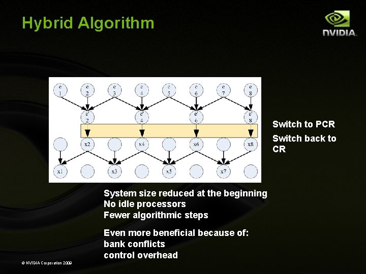
Hybrid Algorithm Switch to PCR Switch back to CR System size reduced at the beginning No idle processors Fewer algorithmic steps Even more beneficial because of: bank conflicts control overhead © NVIDIA Corporation 2009

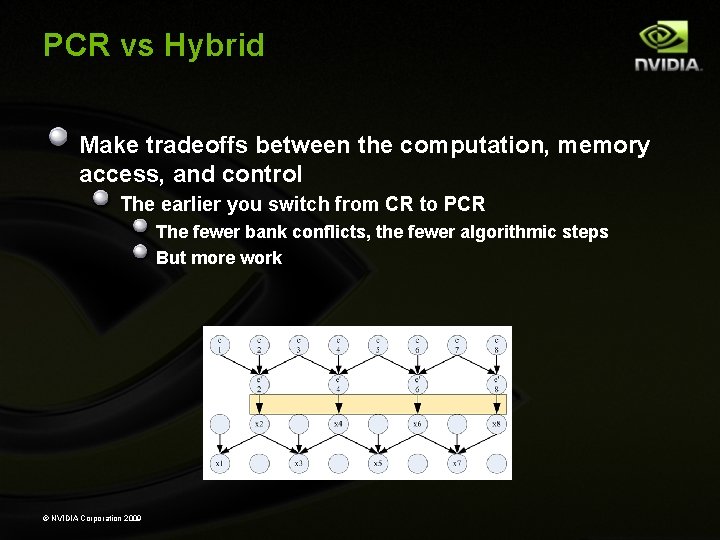
PCR vs Hybrid Make tradeoffs between the computation, memory access, and control The earlier you switch from CR to PCR The fewer bank conflicts, the fewer algorithmic steps But more work © NVIDIA Corporation 2009

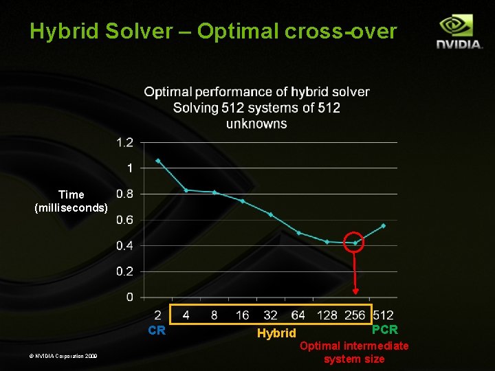
Hybrid Solver – Optimal cross-over Time (milliseconds) CR © NVIDIA Corporation 2009 Hybrid PCR Optimal intermediate system size

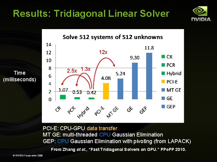
Results: Tridiagonal Linear Solver 12 x 2. 5 x 1. 3 x Time (milliseconds) PCI-E: CPU-GPU data transfer MT GE: multi-threaded CPU Gaussian Elimination GEP: CPU Gaussian Elimination with pivoting (from LAPACK) From Zhang et al. , “Fast Tridiagonal Solvers on GPU. ” PPo. PP 2010. © NVIDIA Corporation 2009

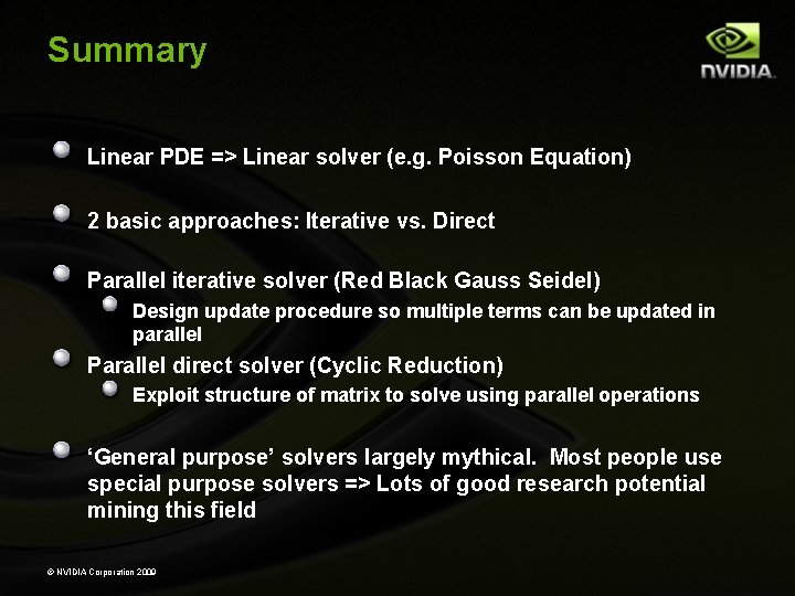
Summary Linear PDE => Linear solver (e. g. Poisson Equation) 2 basic approaches: Iterative vs. Direct Parallel iterative solver (Red Black Gauss Seidel) Design update procedure so multiple terms can be updated in parallel Parallel direct solver (Cyclic Reduction) Exploit structure of matrix to solve using parallel operations ‘General purpose’ solvers largely mythical. Most people use special purpose solvers => Lots of good research potential mining this field © NVIDIA Corporation 2009