Learning to Classify Text William W Cohen Center

Learning to Classify Text William W. Cohen Center for Automated Learning and Discovery Carnegie Mellon University

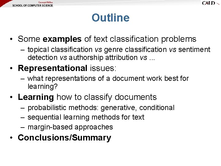
Outline • Some examples of text classification problems – topical classification vs genre classification vs sentiment detection vs authorship attribution vs. . . • Representational issues: – what representations of a document work best for learning? • Learning how to classify documents – probabilistic methods: generative, conditional – sequential learning methods for text – margin-based approaches • Conclusions/Summary

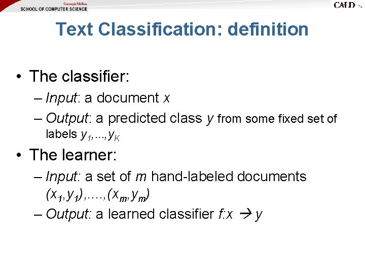
Text Classification: definition • The classifier: – Input: a document x – Output: a predicted class y from some fixed set of labels y 1, . . . , y. K • The learner: – Input: a set of m hand-labeled documents (x 1, y 1), . . , (xm, ym) – Output: a learned classifier f: x y

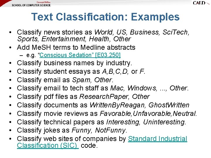
Text Classification: Examples • Classify news stories as World, US, Business, Sci. Tech, Sports, Entertainment, Health, Other • Add Me. SH terms to Medline abstracts – e. g. “Conscious Sedation” [E 03. 250] • • • Classify business names by industry. Classify student essays as A, B, C, D, or F. Classify email as Spam, Other. Classify email to tech staff as Mac, Windows, . . . , Other. Classify pdf files as Research. Paper, Other Classify documents as Written. By. Reagan, Ghost. Written Classify movie reviews as Favorable, Unfavorable, Neutral. Classify technical papers as Interesting, Uninteresting. Classify jokes as Funny, Not. Funny. Classify web sites of companies by Standard Industrial Classification (SIC) code.

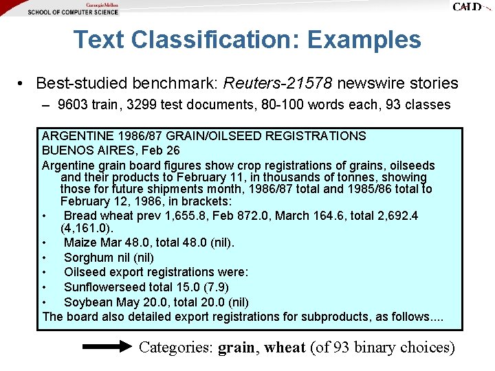
Text Classification: Examples • Best-studied benchmark: Reuters-21578 newswire stories – 9603 train, 3299 test documents, 80 -100 words each, 93 classes ARGENTINE 1986/87 GRAIN/OILSEED REGISTRATIONS BUENOS AIRES, Feb 26 Argentine grain board figures show crop registrations of grains, oilseeds and their products to February 11, in thousands of tonnes, showing those for future shipments month, 1986/87 total and 1985/86 total to February 12, 1986, in brackets: • Bread wheat prev 1, 655. 8, Feb 872. 0, March 164. 6, total 2, 692. 4 (4, 161. 0). • Maize Mar 48. 0, total 48. 0 (nil). • Sorghum nil (nil) • Oilseed export registrations were: • Sunflowerseed total 15. 0 (7. 9) • Soybean May 20. 0, total 20. 0 (nil) The board also detailed export registrations for subproducts, as follows. . Categories: grain, wheat (of 93 binary choices)

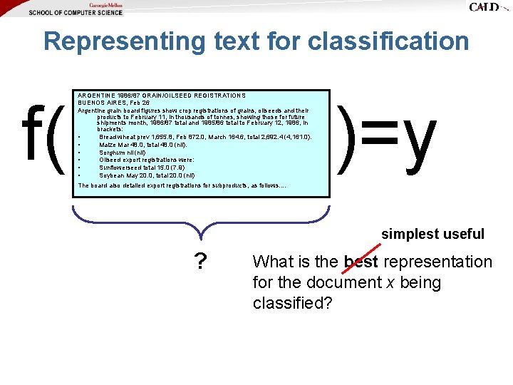
Representing text for classification f( ARGENTINE 1986/87 GRAIN/OILSEED REGISTRATIONS BUENOS AIRES, Feb 26 Argentine grain board figures show crop registrations of grains, oilseeds and their products to February 11, in thousands of tonnes, showing those for future shipments month, 1986/87 total and 1985/86 total to February 12, 1986, in brackets: • Bread wheat prev 1, 655. 8, Feb 872. 0, March 164. 6, total 2, 692. 4 (4, 161. 0). • Maize Mar 48. 0, total 48. 0 (nil). • Sorghum nil (nil) • Oilseed export registrations were: • Sunflowerseed total 15. 0 (7. 9) • Soybean May 20. 0, total 20. 0 (nil) )=y The board also detailed export registrations for subproducts, as follows. . simplest useful ? What is the best representation for the document x being classified?

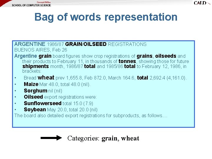
Bag of words representation ARGENTINE 1986/87 GRAIN/OILSEED REGISTRATIONS BUENOS AIRES, Feb 26 Argentine grain board figures show crop registrations of grains, oilseeds and their products to February 11, in thousands of tonnes, showing those for future shipments month, 1986/87 total and 1985/86 total to February 12, 1986, in brackets: • Bread wheat prev 1, 655. 8, Feb 872. 0, March 164. 6, total 2, 692. 4 (4, 161. 0). • Maize Mar 48. 0, total 48. 0 (nil). • Sorghum nil (nil) • Oilseed export registrations were: • Sunflowerseed total 15. 0 (7. 9) • Soybean May 20. 0, total 20. 0 (nil) The board also detailed export registrations for subproducts, as follows. . Categories: grain, wheat

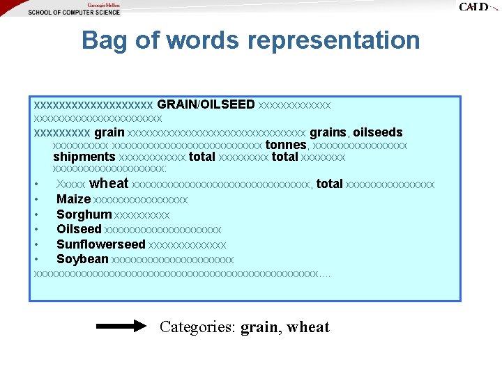
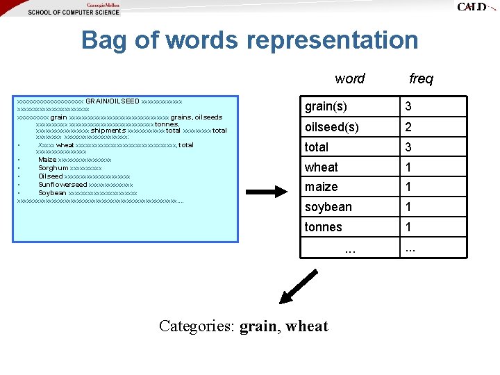
Bag of words representation xxxxxxxxxx GRAIN/OILSEED xxxxxxxxxxxxxxxxxx grain xxxxxxxxxxxxxxxx grains, oilseeds xxxxxxxxxxxxxxxxxxx tonnes, xxxxxxxxx shipments xxxxxx total xxxxxxxxxxxxxx: • Xxxxx wheat xxxxxxxxxxxxxxxx, total xxxxxxxx • Maize xxxxxxxxx • Sorghum xxxxx • Oilseed xxxxxxxxxxx • Sunflowerseed xxxxxxx • Soybean xxxxxxxxxxxxxxxxxxxxxxxxxxxxxxxxxxxxx. . Categories: grain, wheat

Bag of words representation word xxxxxxxxxx GRAIN/OILSEED xxxxxxxxxxxxxxxxxx grain xxxxxxxxxxxxxxxx grains, oilseeds xxxxxxxxxxxxxxxxxxx tonnes, xxxxxxxxx shipments xxxxxx total xxxxxxxxxxxxxx: • Xxxxx wheat xxxxxxxxxxxxxxxx, total xxxxxxxx • Maize xxxxxxxxx • Sorghum xxxxx • Oilseed xxxxxxxxxxx • Sunflowerseed xxxxxxx • Soybean xxxxxxxxxxxxxxxxxxxxxxxxxxxxxxxxxxxxx. . freq grain(s) 3 oilseed(s) 2 total 3 wheat 1 maize 1 soybean 1 tonnes 1 . . . Categories: grain, wheat . . .

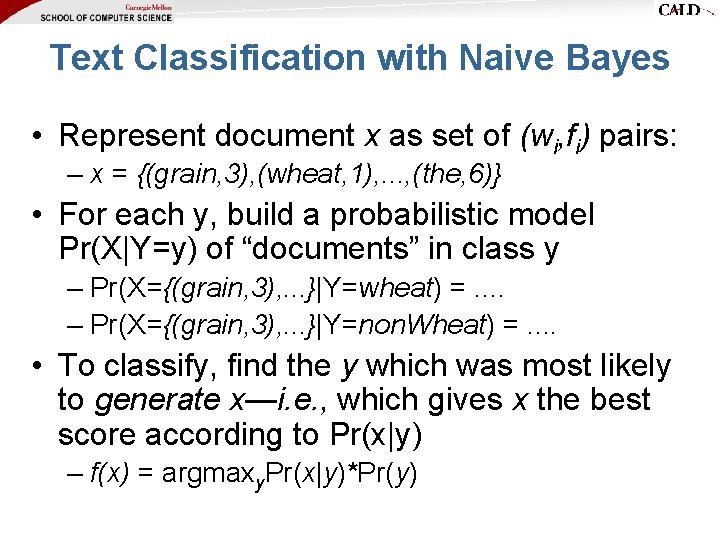
Text Classification with Naive Bayes • Represent document x as set of (wi, fi) pairs: – x = {(grain, 3), (wheat, 1), . . . , (the, 6)} • For each y, build a probabilistic model Pr(X|Y=y) of “documents” in class y – Pr(X={(grain, 3), . . . }|Y=wheat) =. . – Pr(X={(grain, 3), . . . }|Y=non. Wheat) =. . • To classify, find the y which was most likely to generate x—i. e. , which gives x the best score according to Pr(x|y) – f(x) = argmaxy. Pr(x|y)*Pr(y)

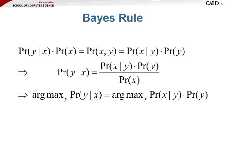
Bayes Rule

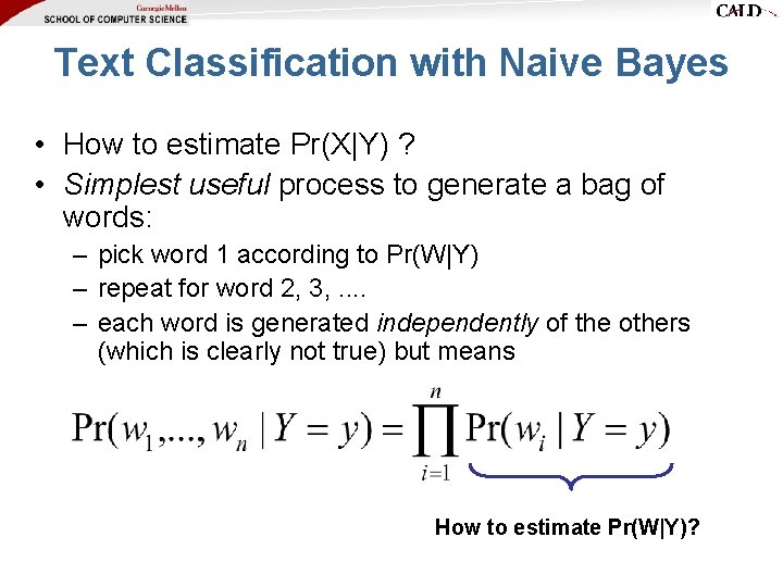
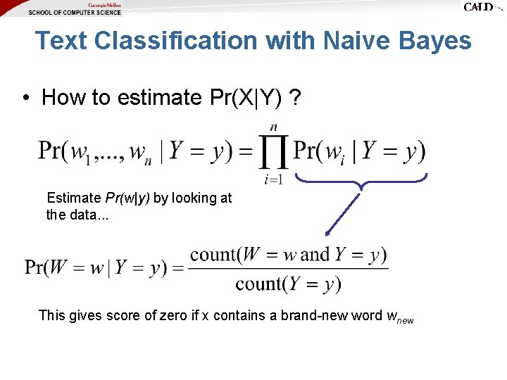
Text Classification with Naive Bayes • How to estimate Pr(X|Y) ? • Simplest useful process to generate a bag of words: – pick word 1 according to Pr(W|Y) – repeat for word 2, 3, . . – each word is generated independently of the others (which is clearly not true) but means How to estimate Pr(W|Y)?

Text Classification with Naive Bayes • How to estimate Pr(X|Y) ? Estimate Pr(w|y) by looking at the data. . . This gives score of zero if x contains a brand-new word wnew

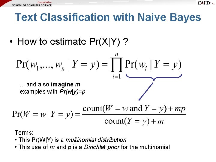
Text Classification with Naive Bayes • How to estimate Pr(X|Y) ? . . . and also imagine m examples with Pr(w|y)=p Terms: • This Pr(W|Y) is a multinomial distribution • This use of m and p is a Dirichlet prior for the multinomial

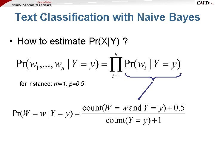
Text Classification with Naive Bayes • How to estimate Pr(X|Y) ? for instance: m=1, p=0. 5

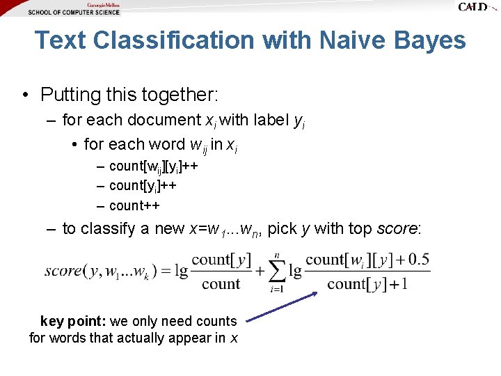
Text Classification with Naive Bayes • Putting this together: – for each document xi with label yi • for each word wij in xi – count[wij][yi]++ – count++ – to classify a new x=w 1. . . wn, pick y with top score: key point: we only need counts for words that actually appear in x

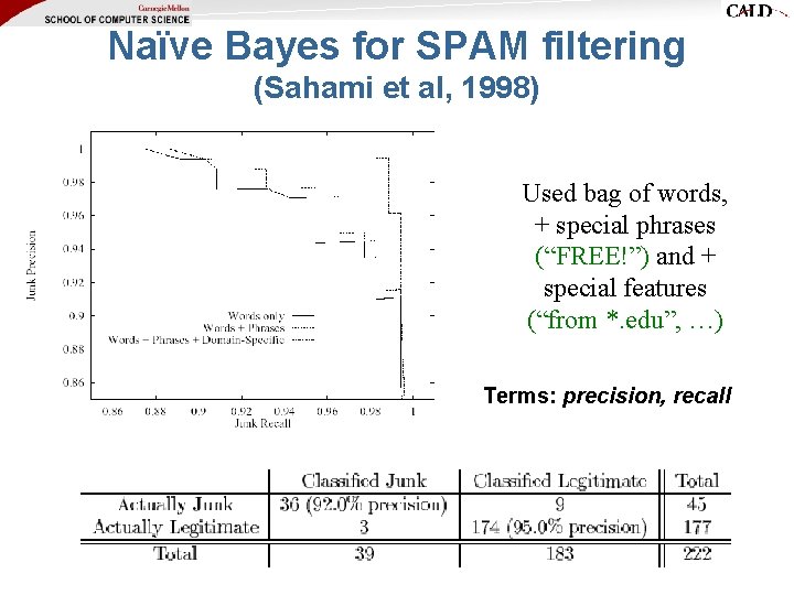
Naïve Bayes for SPAM filtering (Sahami et al, 1998) Used bag of words, + special phrases (“FREE!”) and + special features (“from *. edu”, …) Terms: precision, recall

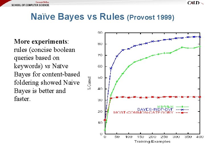
Naïve Bayes vs Rules (Provost 1999) More experiments: rules (concise boolean queries based on keywords) vs Naïve Bayes for content-based foldering showed Naive Bayes is better and faster.

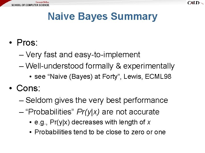
Naive Bayes Summary • Pros: – Very fast and easy-to-implement – Well-understood formally & experimentally • see “Naive (Bayes) at Forty”, Lewis, ECML 98 • Cons: – Seldom gives the very best performance – “Probabilities” Pr(y|x) are not accurate • e. g. , Pr(y|x) decreases with length of x • Probabilities tend to be close to zero or one

Beyond Naive Bayes Non-Multinomial Models Latent Dirichlet Allocation

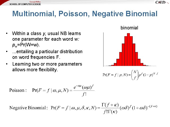
Multinomial, Poisson, Negative Binomial binomial • Within a class y, usual NB learns one parameter for each word w: pw=Pr(W=w). • . . . entailing a particular distribution on word frequencies F. • Learning two or more parameters allows more flexibility.

Multinomial, Poisson, Negative Binomial • Binomial distribution does not fit frequent words or phrases very well. For some tasks frequent words are very important. . . e. g. , classifying text by writing style. – “Who wrote Ronald Reagan’s radio addresses? ”, Airoldi & Fienberg, 2003 • Problem is worse if you consider high-level features extracted from text – Docu. Scope tagger for “semantic markers”

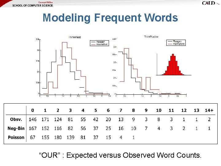
Modeling Frequent Words “OUR” : Expected versus Observed Word Counts.

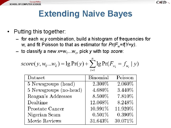
Extending Naive Bayes • Putting this together: – for each w, y combination, build a histogram of frequencies for w, and fit Poisson to that as estimator for Pr(Fw=f|Y=y). – to classify a new x=w 1. . . wn, pick y with top score:

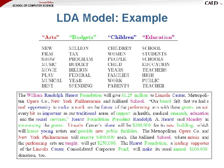
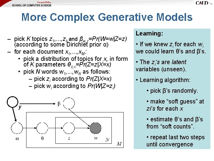
More Complex Generative Models [Blei, Ng & Jordan, JMLR, 2003] • Within a class y, Naive Bayes constructs each x: – pick N words w 1, . . . , w. N according to Pr(W|Y=y) • A more complex model for a class y: – pick K topics z 1, . . . , zk and βw, z=Pr(W=w|Z=z) (according to some Dirichlet prior α) – for each document x: • pick a distribution of topics for X, in form of K parameters θz, x=Pr(Z=z|X=x) • pick N words w 1, . . . , w. N as follows: – pick zi according to Pr(Z|X=x) – pick wi according to Pr(W|Z=zi)

LDA Model: Example

More Complex Generative Models – pick K topics z 1, . . . , zk and βw, z=Pr(W=w|Z=z) (according to some Dirichlet prior α) – for each document x 1, . . . , x. M: • pick a distribution of topics for x, in form of K parameters θz, x=Pr(Z=z|X=x) • pick N words w 1, . . . , w. N as follows: – pick zi according to Pr(Z|X=x) – pick wi according to Pr(W|Z=zi) y Learning: • If we knew zi for each wi we could learn θ’s and β’s. • The zi‘s are latent variables (unseen). • Learning algorithm: • pick β’s randomly. • make “soft guess” at zi‘s for each x • estimate θ’s and β’s from “soft counts”. • repeat last two steps until convergence

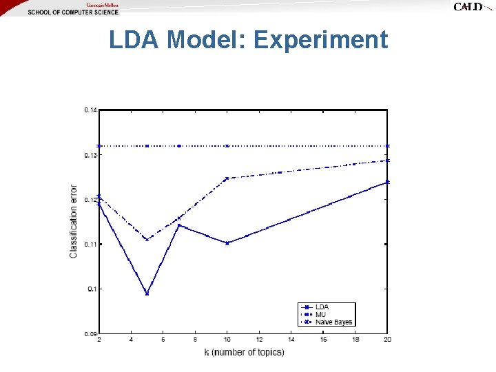
LDA Model: Experiment

Beyond Generative Models Loglinear Conditional Models

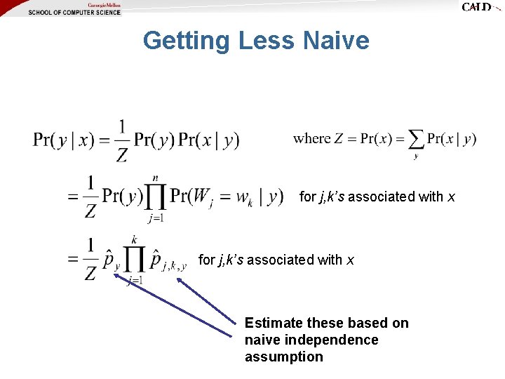
Getting Less Naive for j, k’s associated with x Estimate these based on naive independence assumption

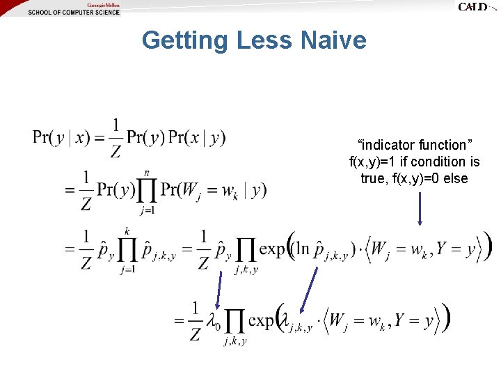
Getting Less Naive “indicator function” f(x, y)=1 if condition is true, f(x, y)=0 else

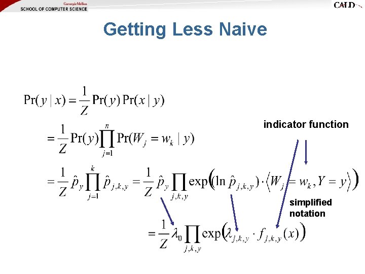
Getting Less Naive indicator function simplified notation

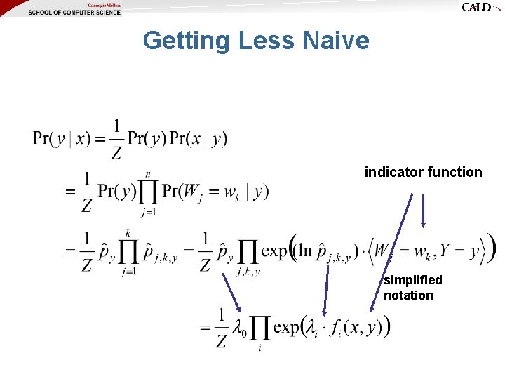
Getting Less Naive indicator function simplified notation

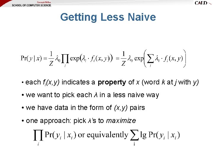
Getting Less Naive • each fi(x, y) indicates a property of x (word k at j with y) • we want to pick each λ in a less naive way • we have data in the form of (x, y) pairs • one approach: pick λ’s to maximize

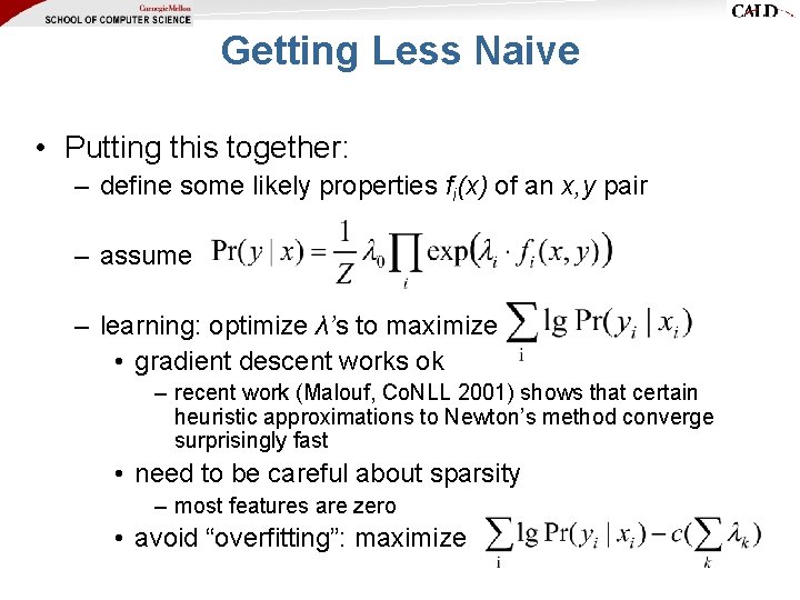
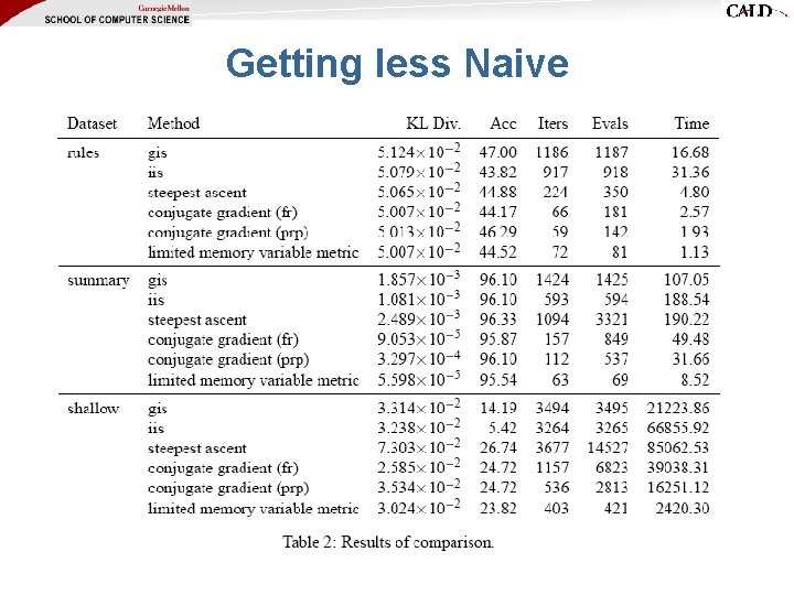
Getting Less Naive • Putting this together: – define some likely properties fi(x) of an x, y pair – assume – learning: optimize λ’s to maximize • gradient descent works ok – recent work (Malouf, Co. NLL 2001) shows that certain heuristic approximations to Newton’s method converge surprisingly fast • need to be careful about sparsity – most features are zero • avoid “overfitting”: maximize

Getting less Naive

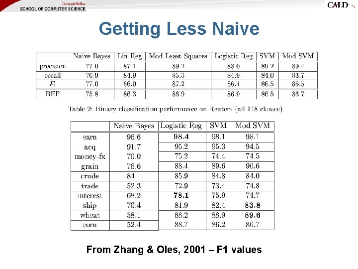
Getting Less Naive From Zhang & Oles, 2001 – F 1 values

HMMs and CRFs

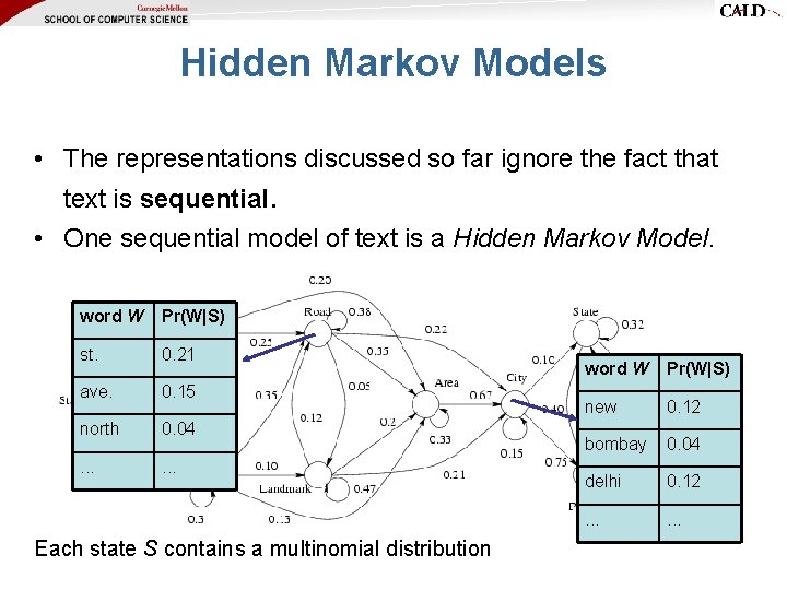
Hidden Markov Models • The representations discussed so far ignore the fact that text is sequential. • One sequential model of text is a Hidden Markov Model. word W Pr(W|S) st. 0. 21 ave. 0. 15 north 0. 04 . . . Each state S contains a multinomial distribution word W Pr(W|S) new 0. 12 bombay 0. 04 delhi 0. 12 . . .

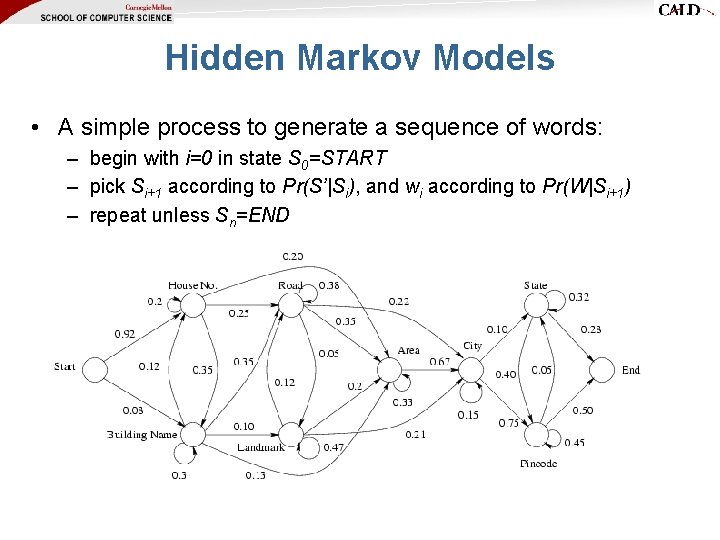
Hidden Markov Models • A simple process to generate a sequence of words: – begin with i=0 in state S 0=START – pick Si+1 according to Pr(S’|Si), and wi according to Pr(W|Si+1) – repeat unless Sn=END

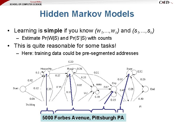
Hidden Markov Models • Learning is simple if you know (w 1, . . . , wn) and (s 1, . . . , sn) – Estimate Pr(W|S) and Pr(S’|S) with counts • This is quite reasonable for some tasks! – Here: training data could be pre-segmented addresses 5000 Forbes Avenue, Pittsburgh PA

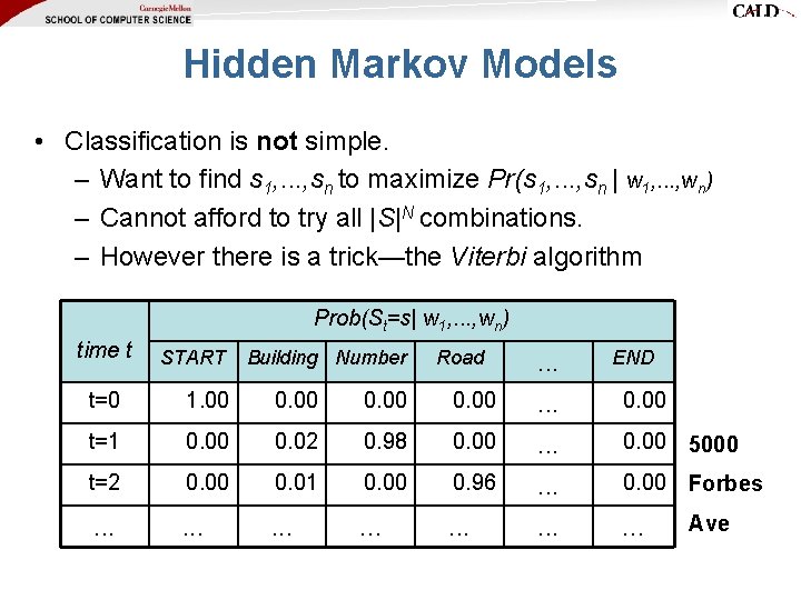
Hidden Markov Models • Classification is not simple. – Want to find s 1, . . . , sn to maximize Pr(s 1, . . . , sn | w 1, . . . , wn) – Cannot afford to try all |S|N combinations. – However there is a trick—the Viterbi algorithm Prob(St=s| w 1, . . . , wn) time t START Building Number Road . . . END t=0 1. 00 0. 00 . . . 0. 00 t=1 0. 00 0. 02 0. 98 0. 00 . . . 0. 00 5000 t=2 0. 00 0. 01 0. 00 0. 96 . . . 0. 00 Forbes . . Ave

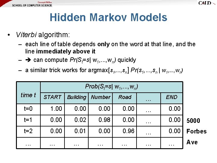
Hidden Markov Models • Viterbi algorithm: – each line of table depends only on the word at that line, and the line immediately above it – can compute Pr(St=s| w 1, . . . , wn) quickly – a similar trick works for argmax[s 1, . . . , sn] Pr(s 1, . . . , sn | w 1, . . . , wn) Prob(St=s| w 1, . . . , wn) time t START Building Number Road . . . END t=0 1. 00 0. 00 . . . 0. 00 t=1 0. 00 0. 02 0. 98 0. 00 . . . 0. 00 5000 t=2 0. 00 0. 01 0. 00 0. 96 . . . 0. 00 Forbes . . Ave

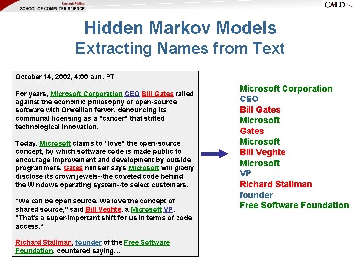
Hidden Markov Models Extracting Names from Text October 14, 2002, 4: 00 a. m. PT For years, Microsoft Corporation CEO Bill Gates railed against the economic philosophy of open-source software with Orwellian fervor, denouncing its communal licensing as a "cancer" that stifled technological innovation. Today, Microsoft claims to "love" the open-source concept, by which software code is made public to encourage improvement and development by outside programmers. Gates himself says Microsoft will gladly disclose its crown jewels--the coveted code behind the Windows operating system--to select customers. "We can be open source. We love the concept of shared source, " said Bill Veghte, a Microsoft VP. "That's a super-important shift for us in terms of code access. “ Richard Stallman, founder of the Free Software Foundation, countered saying… Microsoft Corporation CEO Bill Gates Microsoft Bill Veghte Microsoft VP Richard Stallman founder Free Software Foundation

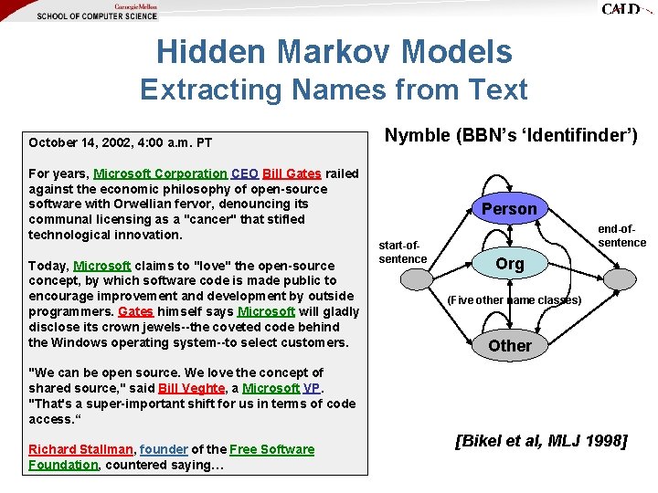
Hidden Markov Models Extracting Names from Text October 14, 2002, 4: 00 a. m. PT For years, Microsoft Corporation CEO Bill Gates railed against the economic philosophy of open-source software with Orwellian fervor, denouncing its communal licensing as a "cancer" that stifled technological innovation. Today, Microsoft claims to "love" the open-source concept, by which software code is made public to encourage improvement and development by outside programmers. Gates himself says Microsoft will gladly disclose its crown jewels--the coveted code behind the Windows operating system--to select customers. Nymble (BBN’s ‘Identifinder’) Person start-ofsentence end-ofsentence Org (Five other name classes) Other "We can be open source. We love the concept of shared source, " said Bill Veghte, a Microsoft VP. "That's a super-important shift for us in terms of code access. “ Richard Stallman, founder of the Free Software Foundation, countered saying… [Bikel et al, MLJ 1998]

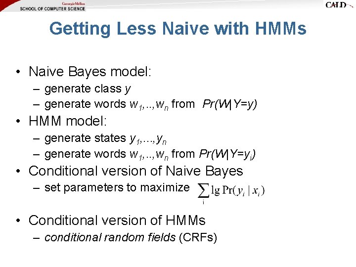
Getting Less Naive with HMMs • Naive Bayes model: – generate class y – generate words w 1, . . , wn from Pr(W|Y=y) • HMM model: – generate states y 1, . . . , yn – generate words w 1, . . , wn from Pr(W|Y=yi) • Conditional version of Naive Bayes – set parameters to maximize • Conditional version of HMMs – conditional random fields (CRFs)

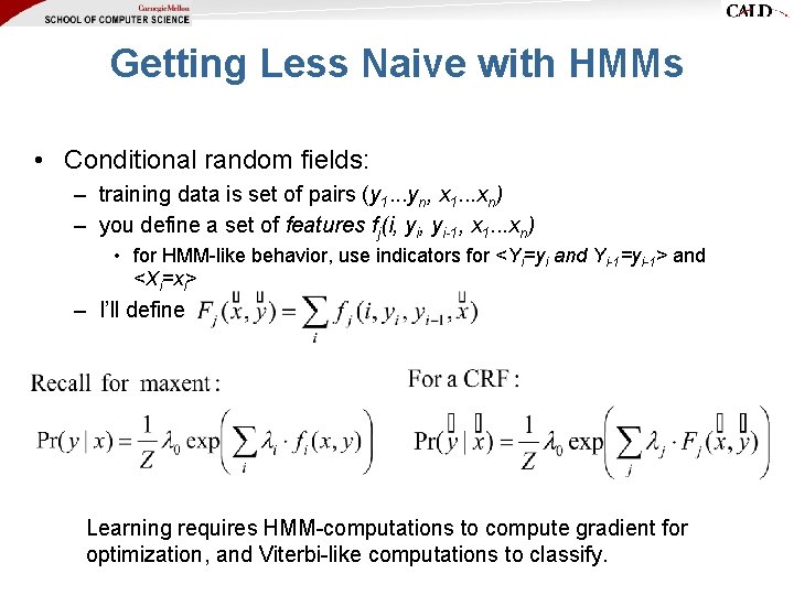
Getting Less Naive with HMMs • Conditional random fields: – training data is set of pairs (y 1. . . yn, x 1. . . xn) – you define a set of features fj(i, yi-1, x 1. . . xn) • for HMM-like behavior, use indicators for <Yi=yi and Yi-1=yi-1> and <Xi=xi> – I’ll define Learning requires HMM-computations to compute gradient for optimization, and Viterbi-like computations to classify.

Experiments with CRFs Learning to Extract Signatures from Email [Carvalho & Cohen, 2004]

CRFs for Shallow Parsing [Sha & Pereira, 2003] in minutes, 375 k examples

Beyond Probabilities

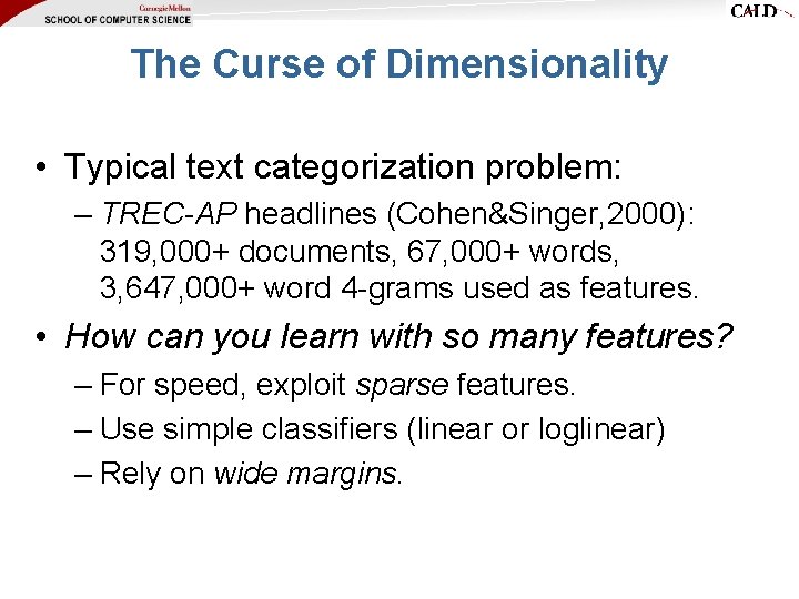
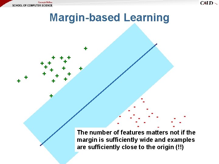
The Curse of Dimensionality • Typical text categorization problem: – TREC-AP headlines (Cohen&Singer, 2000): 319, 000+ documents, 67, 000+ words, 3, 647, 000+ word 4 -grams used as features. • How can you learn with so many features? – For speed, exploit sparse features. – Use simple classifiers (linear or loglinear) – Rely on wide margins.

Margin-based Learning + + ++ + + + -- - - The number of features matters not - - if- the margin is sufficiently wide and examples are sufficiently close to the origin (!!)

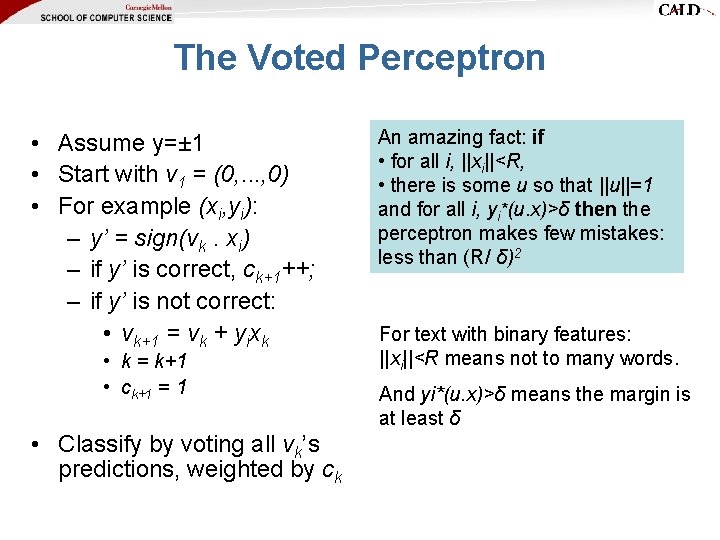
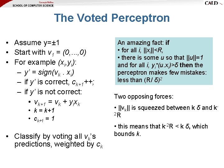
The Voted Perceptron • Assume y=± 1 • Start with v 1 = (0, . . . , 0) • For example (xi, yi): – y’ = sign(vk. xi) – if y’ is correct, ck+1++; – if y’ is not correct: • vk+1 = vk + yixk • k = k+1 • ck+1 = 1 • Classify by voting all vk’s predictions, weighted by ck An amazing fact: if • for all i, ||xi||<R, • there is some u so that ||u||=1 and for all i, yi*(u. x)>δ then the perceptron makes few mistakes: less than (R/ δ)2 For text with binary features: ||xi||<R means not to many words. And yi*(u. x)>δ means the margin is at least δ

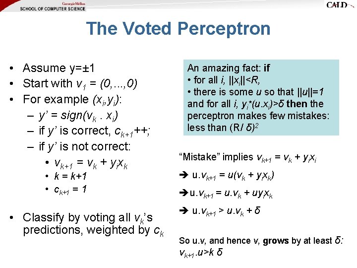
The Voted Perceptron • Assume y=± 1 • Start with v 1 = (0, . . . , 0) • For example (xi, yi): – y’ = sign(vk. xi) – if y’ is correct, ck+1++; – if y’ is not correct: • vk+1 = vk + yixk • k = k+1 • ck+1 = 1 • Classify by voting all vk’s predictions, weighted by ck An amazing fact: if • for all i, ||xi||<R, • there is some u so that ||u||=1 and for all i, yi*(u. xi)>δ then the perceptron makes few mistakes: less than (R/ δ)2 “Mistake” implies vk+1 = vk + yixi u. vk+1 = u(vk + yixk) u. vk+1 = u. vk + uyixk u. vk+1 > u. vk + δ So u. v, and hence v, grows by at least δ: vk+1. u>k δ

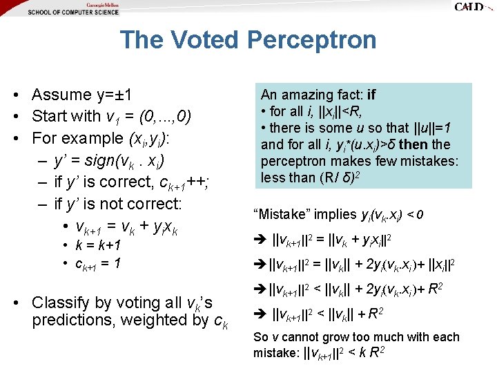
The Voted Perceptron • Assume y=± 1 • Start with v 1 = (0, . . . , 0) • For example (xi, yi): – y’ = sign(vk. xi) – if y’ is correct, ck+1++; – if y’ is not correct: • vk+1 = vk + yixk • k = k+1 • ck+1 = 1 • Classify by voting all vk’s predictions, weighted by ck An amazing fact: if • for all i, ||xi||<R, • there is some u so that ||u||=1 and for all i, yi*(u. xi)>δ then the perceptron makes few mistakes: less than (R/ δ)2 “Mistake” implies yi(vk. xi) < 0 ||vk+1||2 = ||vk + yixi||2 ||vk+1||2 = ||vk|| + 2 yi(vk. xi )+ ||xi||2 ||vk+1||2 < ||vk|| + 2 yi(vk. xi )+ R 2 ||vk+1||2 < ||vk|| + R 2 So v cannot grow too much with each mistake: ||vk+1||2 < k R 2

The Voted Perceptron • Assume y=± 1 • Start with v 1 = (0, . . . , 0) • For example (xi, yi): – y’ = sign(vk. xi) – if y’ is correct, ck+1++; – if y’ is not correct: • vk+1 = vk + yixk • k = k+1 • ck+1 = 1 • Classify by voting all vk’s predictions, weighted by ck An amazing fact: if • for all i, ||xi||<R, • there is some u so that ||u||=1 and for all i, yi*(u. xi)>δ then the perceptron makes few mistakes: less than (R/ δ)2 Two opposing forces: • ||vk|| is squeezed between k δ and k 2 R • this means that k-2 R < k δ, which bounds k.

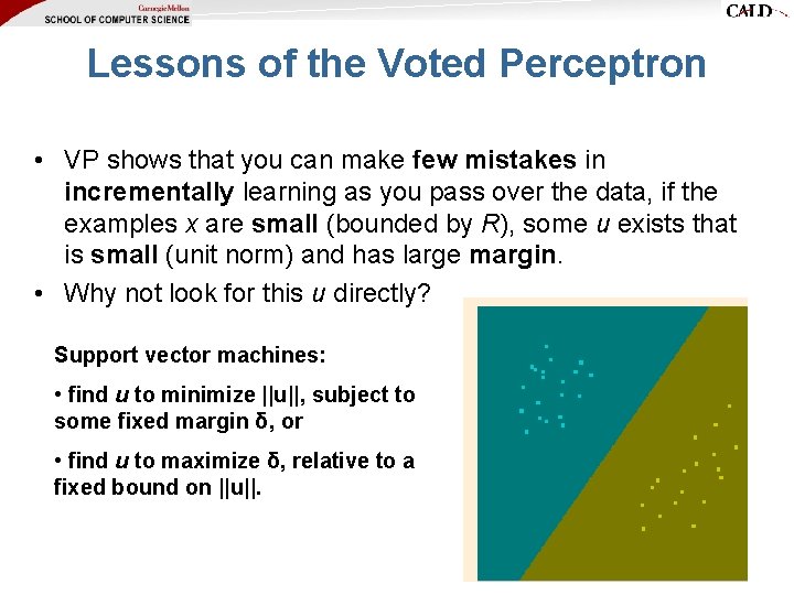
Lessons of the Voted Perceptron • VP shows that you can make few mistakes in incrementally learning as you pass over the data, if the examples x are small (bounded by R), some u exists that is small (unit norm) and has large margin. • Why not look for this u directly? Support vector machines: • find u to minimize ||u||, subject to some fixed margin δ, or • find u to maximize δ, relative to a fixed bound on ||u||.

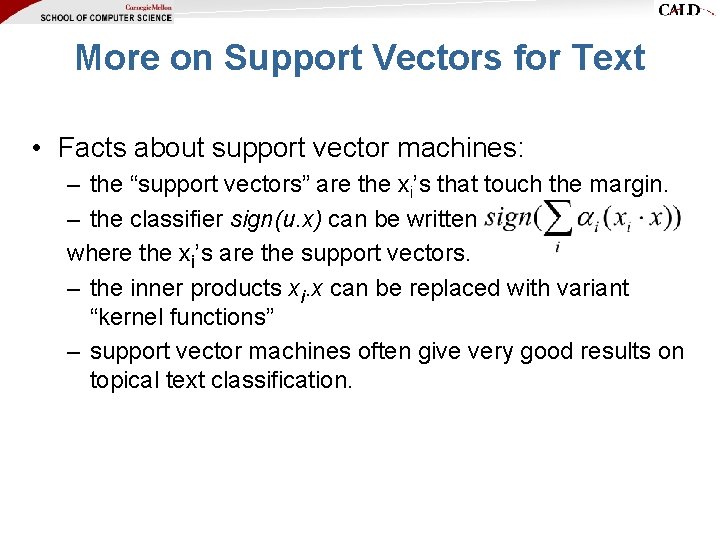
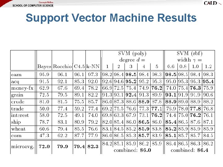
More on Support Vectors for Text • Facts about support vector machines: – the “support vectors” are the xi’s that touch the margin. – the classifier sign(u. x) can be written where the xi’s are the support vectors. – the inner products xi. x can be replaced with variant “kernel functions” – support vector machines often give very good results on topical text classification.

Support Vector Machine Results

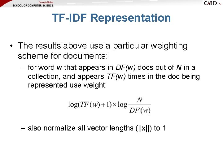
TF-IDF Representation • The results above use a particular weighting scheme for documents: – for word w that appears in DF(w) docs out of N in a collection, and appears TF(w) times in the doc being represented use weight: – also normalize all vector lengths (||x||) to 1

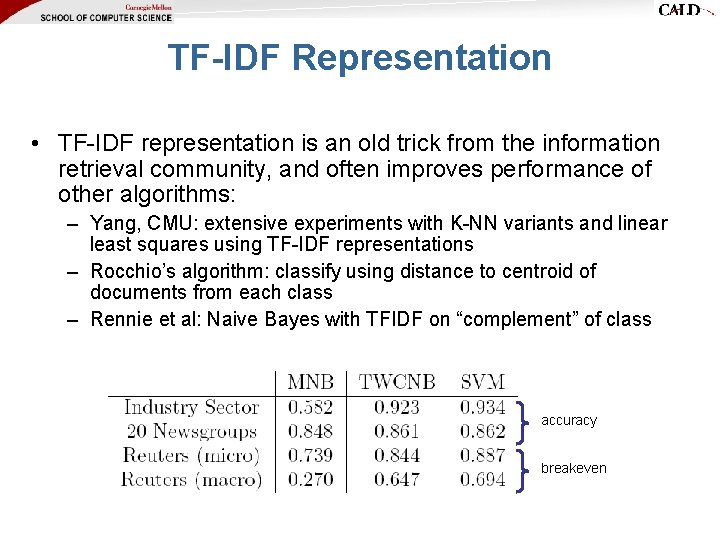
TF-IDF Representation • TF-IDF representation is an old trick from the information retrieval community, and often improves performance of other algorithms: – Yang, CMU: extensive experiments with K-NN variants and linear least squares using TF-IDF representations – Rocchio’s algorithm: classify using distance to centroid of documents from each class – Rennie et al: Naive Bayes with TFIDF on “complement” of class accuracy breakeven

Conclusions • There are huge number of applications for text categorization. • Bag-of-words representations generally work better than you’d expect – Naive Bayes and voted perceptron are fastest to learn and easiest to implement – Linear classifiers that like wide margins tend to do best. – Probabilistic classifications are sometimes important. • Non-topical text categorization (e. g. , sentiment detection) is much less well studied than topic text categorization.

Some Resources for Text Categorization • Surveys and talks: – Machine Learning in Automated Text Categorization, Fabrizio Sebastiani, ACM Computing Surveys, 34(1): 1 -47, 2002 , http: //faure. isti. cnr. it/~fabrizio/Publications/ACMCS 02. pdf – (Naive) Bayesian Text Classification for Spam Filtering http: //www. daviddlewis. com/publications/slides/lewis-2004 -0507 -spam-talkfor-casa-marketing-draft 5. ppt (and other related talks) • Software: – Minorthird: toolkit for extraction and classification of text: http: //minorthird. sourceforge. net – Rainbow: fast Naive Bayes implementation of text-preprocessing in C: http: //www. cs. cmu. edu/~mccallum/bow/rainbow/ – SVM Light: free support vector machine well-suited to text: http: //svmlight. joachims. org/ • Test Data: – Datasets: http: //www. cs. cmu. edu/~tom/, and http: //www. daviddlewis. com/resources/testcollections

Papers Discussed • Naive Bayes for Text: – A Bayesian approach to filtering junk e-mail. M. Sahami, S. Dumais, D. Heckerman, and E. Horvitz (1998). AAAI'98 Workshop on Learning for Text Categorization, July 27, 1998, Madison, Wisconsin. – Machine Learning, Tom Mitchell, Mc. Graw Hill, 1997. – Naive-Bayes vs. Rule-Learning in Classification of Email. Provost, J (1999). The University of Texas at Austin, Artificial Intelligence Lab. Technical Report AI-TR-99 -284 – Naive (Bayes) at Forty: The Independence Assumption in Information Retrieval, David Lewis, Proceedings of the 10 th European Conference on Machine Learning, 1998 • • • Extensions to Naive Bayes: – Who Wrote Ronald Reagan's Radio Addresses ? E. Airoldi and S. Fienberg (2003), CMU statistics dept TR, http: //www. stat. cmu. edu/tr/tr 789. html – Latent Dirichlet allocation. D. Blei, A. Ng, and M. Jordan. Journal of Machine Learning Research, 3: 993 -1022, January 2003 – Tackling the Poor Assumptions of Naive Bayes Text Classifiers Jason D. M. Rennie, Lawrence Shih, Jaime Teevan and David R. Karger. Proceedings of the Twentieth International Conference on Machine Learning. 2003 Max. Ent and SVMs: – A comparison of algorithms for maximum entropy parameter estimation. Robert Malouf, 2002. In Proceedings of the Sixth Conference on Natural Language Learning (Co. NLL-2002). Pages 49 -55. – Text categorization based on regularized linear classification methods. Tong Zhang and Frank J. Oles. Information Retrieval, 4: 5 -31, 2001. – Learning to Classify Text using Support Vector Machines, T. Joachims, Kluwer, 2002. HMMs and CRFs: – Automatic segmentation of text into structured records, Borkar et al, SIGMOD 2001 – Learning to Extract Signature and Reply Lines from Email, Carvalo & Cohen, in Conference on Email and Anti-Spam 2004 – Shallow Parsing with Conditional Random Fields. F. Sha and F. Pereira. HLT-NAACL, 2003