III Completely Randomized Design CRD III A Design

III. Completely Randomized Design (CRD) III. A Design of a CRD III. B Models and estimation for a CRD III. C Hypothesis testing using the ANOVA method III. D Diagnostic checking III. E Treatment differences Statistical Modelling Chapter III 1

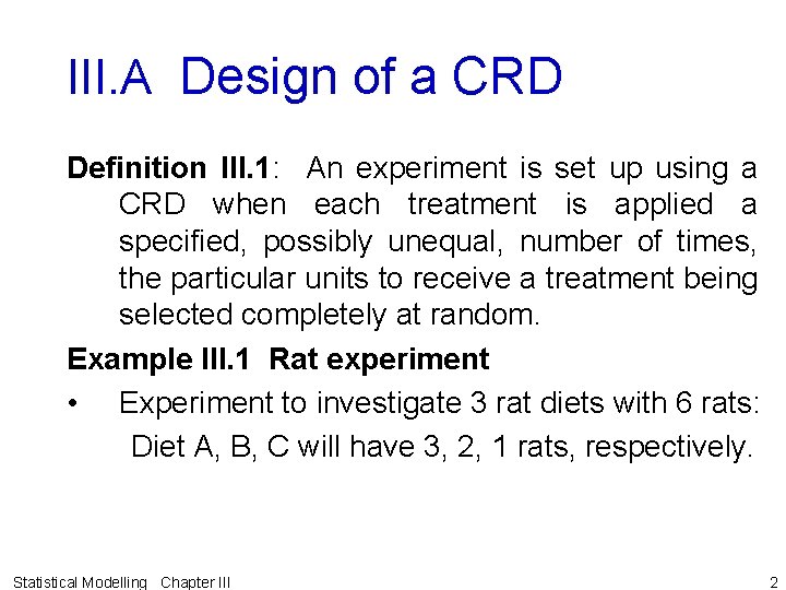
III. A Design of a CRD Definition III. 1: An experiment is set up using a CRD when each treatment is applied a specified, possibly unequal, number of times, the particular units to receive a treatment being selected completely at random. Example III. 1 Rat experiment • Experiment to investigate 3 rat diets with 6 rats: Diet A, B, C will have 3, 2, 1 rats, respectively. Statistical Modelling Chapter III 2

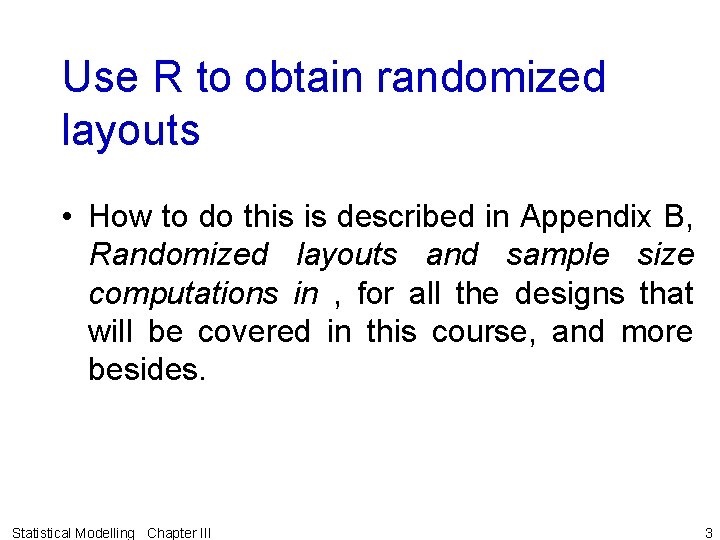
Use R to obtain randomized layouts • How to do this is described in Appendix B, Randomized layouts and sample size computations in , for all the designs that will be covered in this course, and more besides. Statistical Modelling Chapter III 3

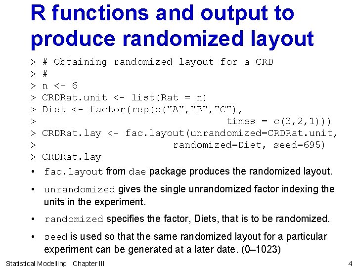
R functions and output to produce randomized layout > # Obtaining randomized layout for a CRD > # > n <- 6 > CRDRat. unit <- list(Rat = n) > Diet <- factor(rep(c("A", "B", "C"), > times = c(3, 2, 1))) > CRDRat. lay <- fac. layout(unrandomized=CRDRat. unit, > randomized=Diet, seed=695) > CRDRat. lay • fac. layout from dae package produces the randomized layout. • unrandomized gives the single unrandomized factor indexing the units in the experiment. • randomized specifies the factor, Diets, that is to be randomized. • seed is used so that the same randomized layout for a particular experiment can be generated at a later date. (0– 1023) Statistical Modelling Chapter III 4

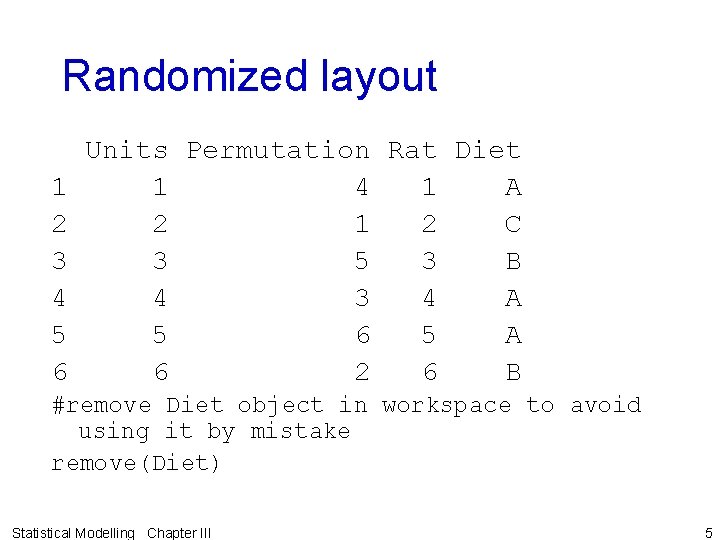
Randomized layout Units Permutation Rat Diet 1 1 4 1 A 2 2 1 2 C 3 3 5 3 B 4 4 3 4 A 5 5 6 5 A 6 6 2 6 B #remove Diet object in workspace to avoid using it by mistake remove(Diet) Statistical Modelling Chapter III 5

III. B Models and estimation for a CRD • The analysis of CRD experiments uses: – least-squares or maximum likelihood estimation of the parameters of a linear model – hypothesis testing based on the ANOVA method or maximum likelihood ratio testing. • Use rat experiment to investigate linear models and the estimation of its parameters. Statistical Modelling Chapter III 6

a) Maximal model • Definition III. 2: The maximal expectation model is the most complicated model for the expectation that is to be considered in analysing an experiment. • We first consider the maximal model for the CRD. Statistical Modelling Chapter III 7

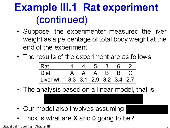
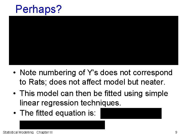
Example III. 1 Rat experiment (continued) • Suppose, the experimenter measured the liver weight as a percentage of total body weight at the end of the experiment. • The results of the experiment are as follows: • The analysis based on a linear model, that is: • Our model also involves assuming • Trick is what are X and q going to be? Statistical Modelling Chapter III 8

Perhaps? • Note numbering of Y's does not correspond to Rats; does not affect model but neater. • This model can then be fitted using simple linear regression techniques. • The fitted equation is: Statistical Modelling Chapter III 9

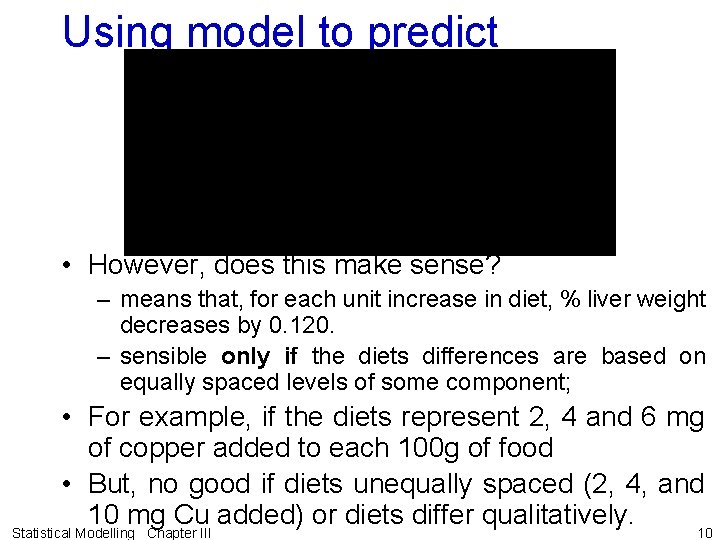
Using model to predict • However, does this make sense? – means that, for each unit increase in diet, % liver weight decreases by 0. 120. – sensible only if the diets differences are based on equally spaced levels of some component; • For example, if the diets represent 2, 4 and 6 mg of copper added to each 100 g of food • But, no good if diets unequally spaced (2, 4, and 10 mg Cu added) or diets differ qualitatively. 10 Statistical Modelling Chapter III

Regression on indicator variables • In this method the explanatory variables are called factors and the possible values they take levels. • Thus, we have a factor Diet with 3 levels: A, B, C. • Definition III. 3: Indicator variables are formed from a factor: – create a variable for each level of the factor; – the values of a variable are either 1 or 0, 1 when the unit has the particular level for that variable and 0 otherwise. Statistical Modelling Chapter III 11

Indicator-variable model • Hence E[Yi] ak, var[Yi] s 2, cov[Yi, Yj] 0, (i j) • Can be written as • Model suggests 3 different expected (or mean) values for the diets. Statistical Modelling Chapter III 12

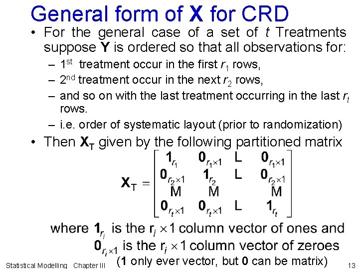
General form of X for CRD • For the general case of a set of t Treatments suppose Y is ordered so that all observations for: – 1 st treatment occur in the first r 1 rows, – 2 nd treatment occur in the next r 2 rows, – and so on with the last treatment occurring in the last rt rows. – i. e. order of systematic layout (prior to randomization) • Then XT given by the following partitioned matrix Statistical Modelling Chapter III (1 only ever vector, but 0 can be matrix) 13

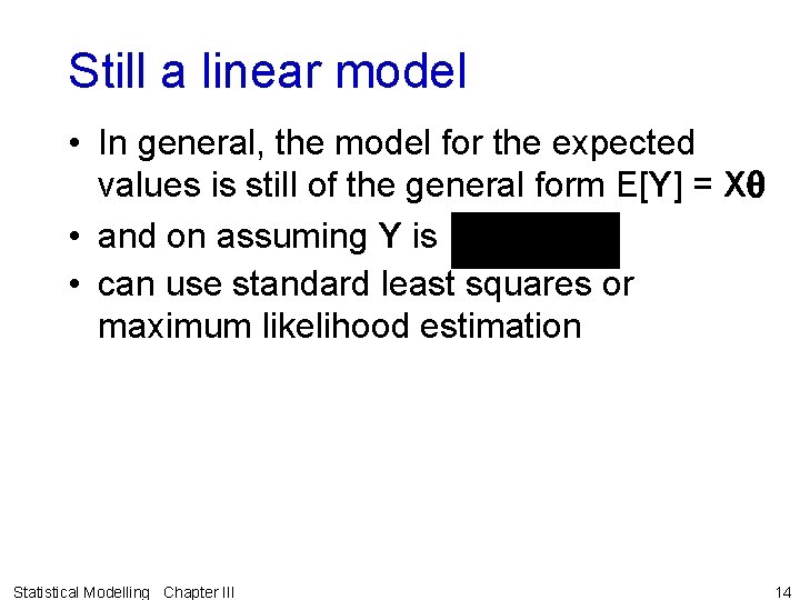
Still a linear model • In general, the model for the expected values is still of the general form E[Y] = Xq • and on assuming Y is • can use standard least squares or maximum likelihood estimation Statistical Modelling Chapter III 14

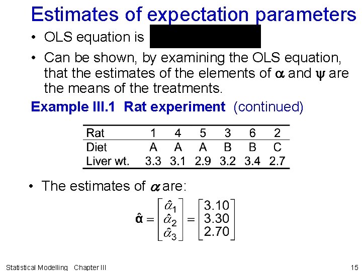
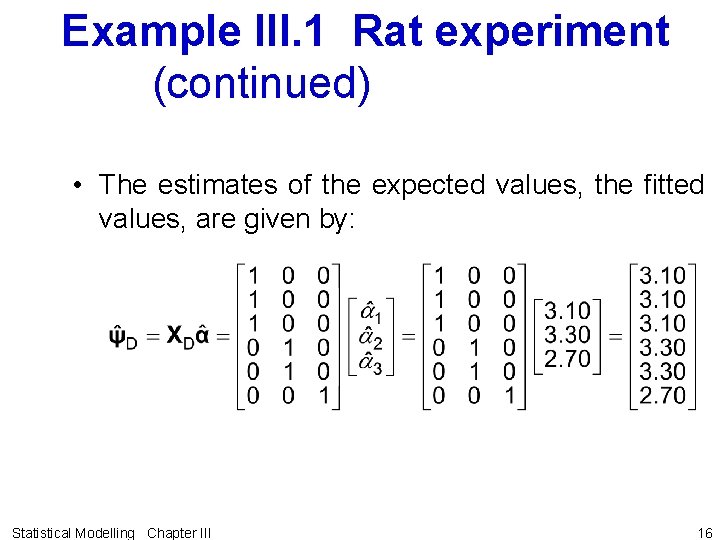
Estimates of expectation parameters • OLS equation is • Can be shown, by examining the OLS equation, that the estimates of the elements of a and y are the means of the treatments. Example III. 1 Rat experiment (continued) • The estimates of a are: Statistical Modelling Chapter III 15

Example III. 1 Rat experiment (continued) • The estimates of the expected values, the fitted values, are given by: Statistical Modelling Chapter III 16

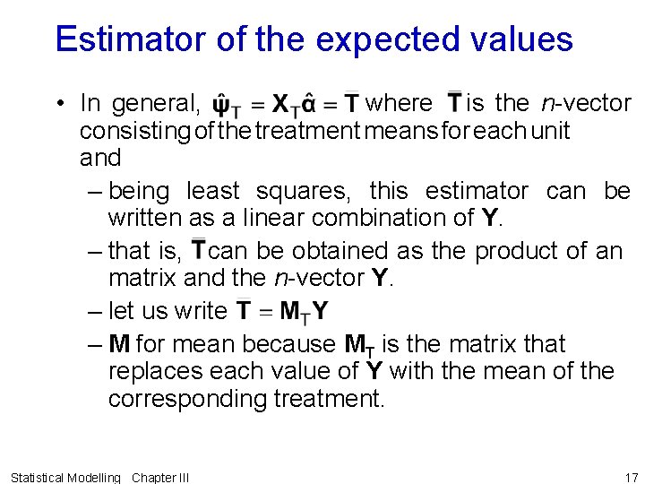
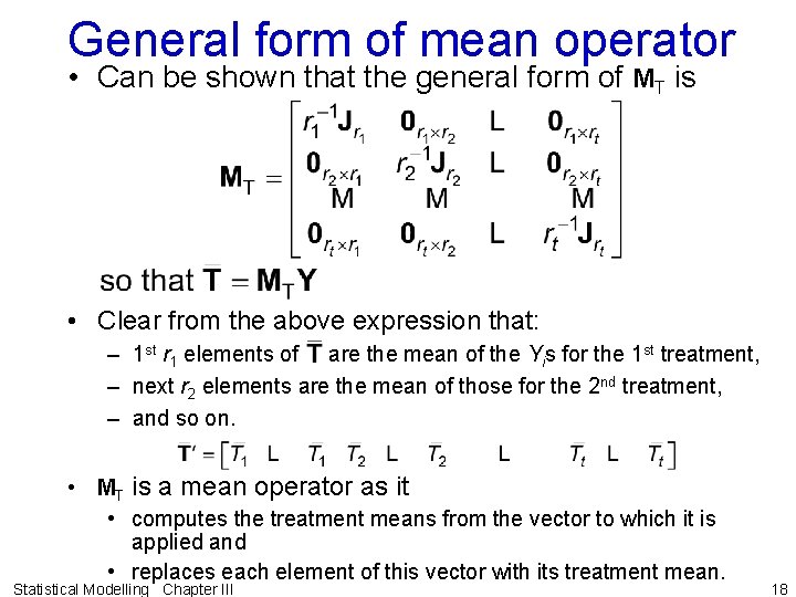
Estimator of the expected values • In general, where is the n-vector consisting of the treatment means for each unit and – being least squares, this estimator can be written as a linear combination of Y. – that is, can be obtained as the product of an matrix and the n-vector Y. – let us write – M for mean because MT is the matrix that replaces each value of Y with the mean of the corresponding treatment. Statistical Modelling Chapter III 17

General form of mean operator • Can be shown that the general form of MT is • Clear from the above expression that: – 1 st r 1 elements of are the mean of the Yis for the 1 st treatment, – next r 2 elements are the mean of those for the 2 nd treatment, – and so on. • MT is a mean operator as it • computes the treatment means from the vector to which it is applied and • replaces each element of this vector with its treatment mean. Statistical Modelling Chapter III 18

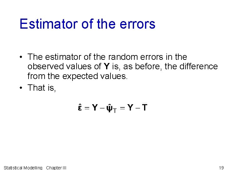
Estimator of the errors • The estimator of the random errors in the observed values of Y is, as before, the difference from the expected values. • That is, Statistical Modelling Chapter III 19

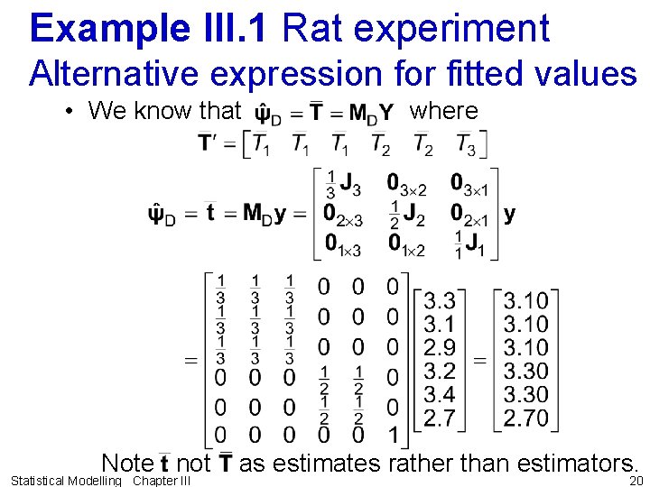
Example III. 1 Rat experiment Alternative expression for fitted values • We know that where Note not as estimates rather than estimators. Statistical Modelling Chapter III 20

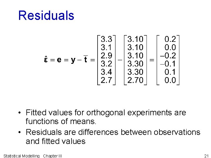
Residuals • Fitted values for orthogonal experiments are functions of means. • Residuals are differences between observations and fitted values Statistical Modelling Chapter III 21

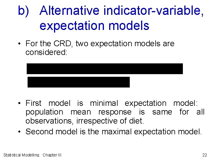
b) Alternative indicator-variable, expectation models • For the CRD, two expectation models are considered: • First model is minimal expectation model: population mean response is same for all observations, irrespective of diet. • Second model is the maximal expectation model. Statistical Modelling Chapter III 22

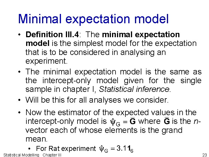
Minimal expectation model • Definition III. 4: The minimal expectation model is the simplest model for the expectation that is to be considered in analysing an experiment. • The minimal expectation model is the same as the intercept-only model given for the single sample in chapter I, Statistical inference. • Will be this for all analyses we consider. • Now the estimator of the expected values in the intercept-only model is where is the nvector each of whose elements is the grand mean. • For Rat experiment Statistical Modelling Chapter III 23

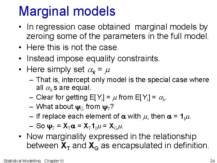
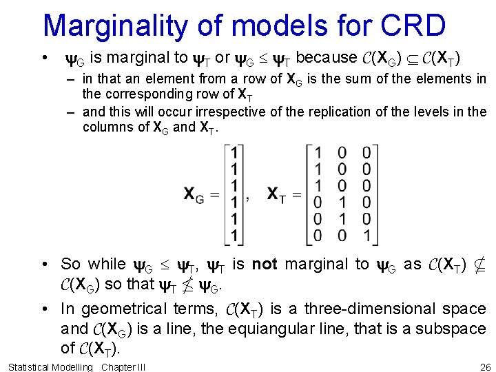
Marginal models • In regression case obtained marginal models by zeroing some of the parameters in the full model. • Here this is not the case. • Instead impose equality constraints. • Here simply set ak = m – That is, intercept only model is the special case where all ak s are equal. – Clear for getting E[Yi] = m from E[Yi] = ak. – What about y. G from y. T? – If replace each element of a with m, then a = 1 tm. – So y. T = XTa = XT 1 tm = XGm. • Now marginality expressed in the relationship between XT and XG as encapsulated in definition. Statistical Modelling Chapter III 24

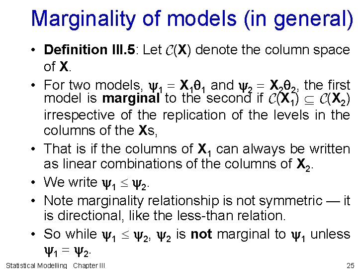
Marginality of models (in general) • Definition III. 5: Let C(X) denote the column space of X. • For two models, y 1 X 1 q 1 and y 2 X 2 q 2, the first model is marginal to the second if C(X 1) C(X 2) irrespective of the replication of the levels in the columns of the Xs, • That is if the columns of X 1 can always be written as linear combinations of the columns of X 2. • We write y 1 y 2. • Note marginality relationship is not symmetric — it is directional, like the less-than relation. • So while y 1 y 2, y 2 is not marginal to y 1 unless y 1 y 2. Statistical Modelling Chapter III 25

Marginality of models for CRD • y. G is marginal to y. T or y. G y. T because C(XG) C(XT) – in that an element from a row of XG is the sum of the elements in the corresponding row of XT – and this will occur irrespective of the replication of the levels in the columns of XG and XT. • So while y. G y. T, y. T is not marginal to y. G as C(XT) C(XG) so that y. T y. G. • In geometrical terms, C(XT) is a three-dimensional space and C(XG) is a line, the equiangular line, that is a subspace of C(XT). Statistical Modelling Chapter III 26

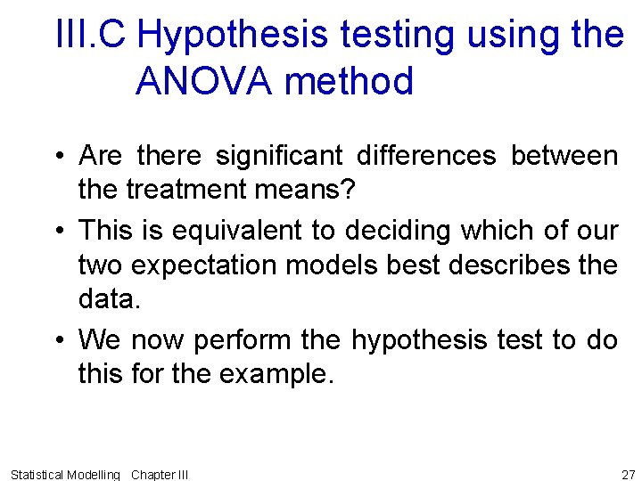
III. C Hypothesis testing using the ANOVA method • Are there significant differences between the treatment means? • This is equivalent to deciding which of our two expectation models best describes the data. • We now perform the hypothesis test to do this for the example. Statistical Modelling Chapter III 27

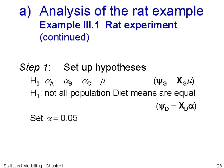
a) Analysis of the rat example Example III. 1 Rat experiment (continued) Step 1: Set up hypotheses H 0: a. A a. B a. C m (y. G XGm) H 1: not all population Diet means are equal (y. D XDa) Set a 0. 05 Statistical Modelling Chapter III 28

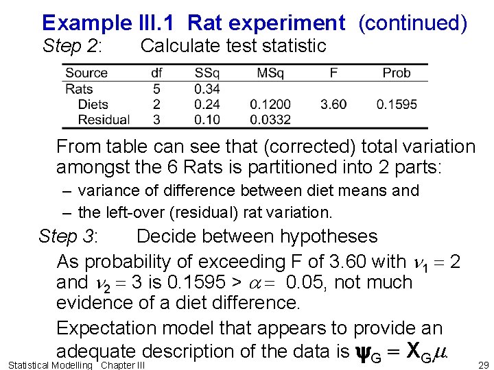
Example III. 1 Rat experiment (continued) Step 2: Calculate test statistic From table can see that (corrected) total variation amongst the 6 Rats is partitioned into 2 parts: – variance of difference between diet means and – the left-over (residual) rat variation. Step 3: Decide between hypotheses As probability of exceeding F of 3. 60 with n 1 2 and n 2 3 is 0. 1595 > a 0. 05, not much evidence of a diet difference. Expectation model that appears to provide an adequate description of the data is y. G XGm. Statistical Modelling Chapter III 29

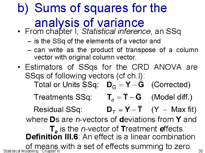
b) Sums of squares for the analysis of variance • From chapter I, Statistical inference, an SSq – is the SSq of the elements of a vector and – can write as the product of transpose of a column vector with original column vector. • Estimators of SSqs for the CRD ANOVA are SSqs of following vectors (cf ch. I): where Ds are n-vectors of deviations from Y and Te is the n-vector of Treatment effects. Definition III. 6: An effect is a linear combination of means with a set of effects summing to zero. 30 Statistical Modelling Chapter III

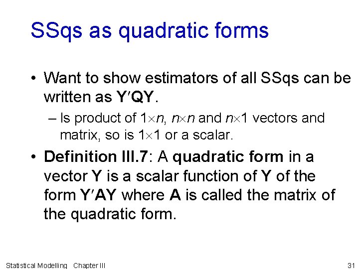
SSqs as quadratic forms • Want to show estimators of all SSqs can be written as Y QY. – Is product of 1 n, n n and n 1 vectors and matrix, so is 1 1 or a scalar. • Definition III. 7: A quadratic form in a vector Y is a scalar function of Y of the form Y AY where A is called the matrix of the quadratic form. Statistical Modelling Chapter III 31

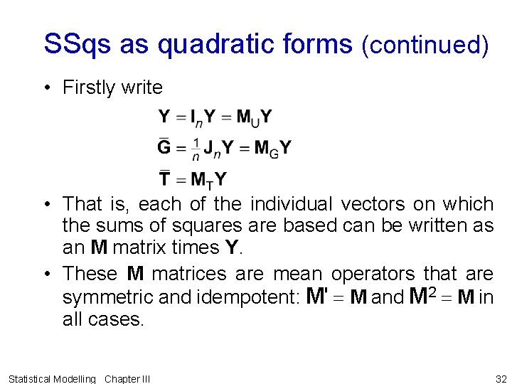
SSqs as quadratic forms (continued) • Firstly write • That is, each of the individual vectors on which the sums of squares are based can be written as an M matrix times Y. • These M matrices are mean operators that are symmetric and idempotent: M' M and M 2 M in all cases. Statistical Modelling Chapter III 32

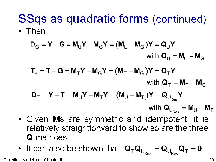
SSqs as quadratic forms (continued) • Then • Given Ms are symmetric and idempotent, it is relatively straightforward to show so are three Q matrices. • It can also be shown that Statistical Modelling Chapter III 33

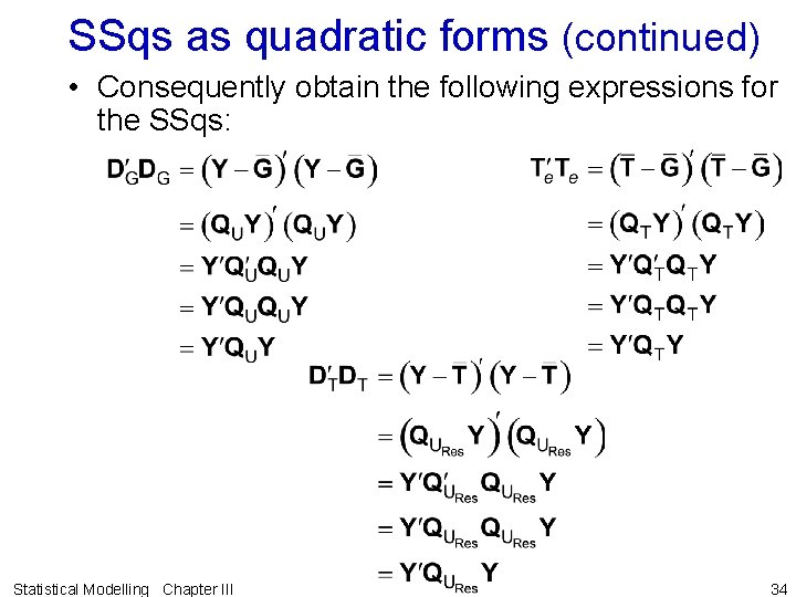
SSqs as quadratic forms (continued) • Consequently obtain the following expressions for the SSqs: Statistical Modelling Chapter III 34

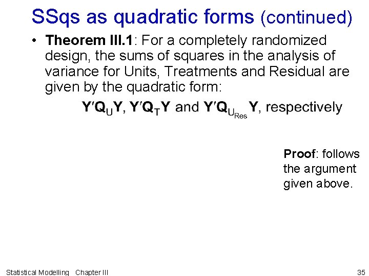
SSqs as quadratic forms (continued) • Theorem III. 1: For a completely randomized design, the sums of squares in the analysis of variance for Units, Treatments and Residual are given by the quadratic form: Proof: follows the argument given above. Statistical Modelling Chapter III 35

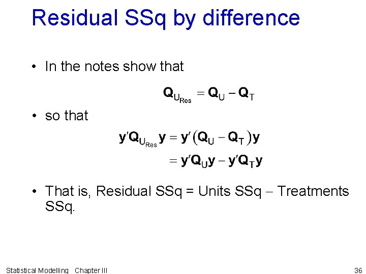
Residual SSq by difference • In the notes show that • so that • That is, Residual SSq = Units SSq - Treatments SSq. Statistical Modelling Chapter III 36

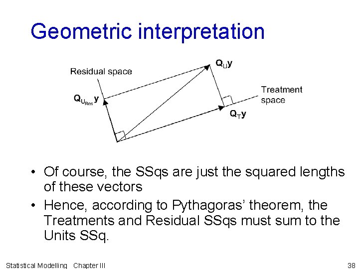
ANOVA table construction • As in regression, Qs are orthogonal projection matrices. – QU orthogonally projects the data vector into the n-1 dimensional part of the n-dimensional data space that is orthogonal to equiangular line. – QT orthogonally projects data vector into the t-1 dimensional part of the t-dimensional Treatment space, that is orthogonal to equiangular line. (Here the Treatment space is the column space of XT. ) – Finally, the matrix orthogonally projects the data vector into the n-t dimensional Residual subspace. – That is, Units space is divided into the two orthogonal subspaces, the Treatments and Residual subspaces. Statistical Modelling Chapter III 37

Geometric interpretation • Of course, the SSqs are just the squared lengths of these vectors • Hence, according to Pythagoras’ theorem, the Treatments and Residual SSqs must sum to the Units SSq. Statistical Modelling Chapter III 38

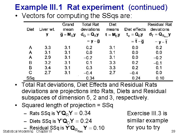
Example III. 1 Rat experiment (continued) • Vectors for computing the SSqs are: • Total Rat deviations, Diet Effects and Residual Rats deviations are projections into Rats, Diets and Residual subspaces of dimension 5, 2 and 3, respectively. • Squared length of projection = SSq – Rats SSq is Y'QRY 0. 34 Exercise III. 3 is similar example – Diets SSq is Y'QDY 0. 24 for you to try – Residual SSq is Statistical Modelling Chapter III 39

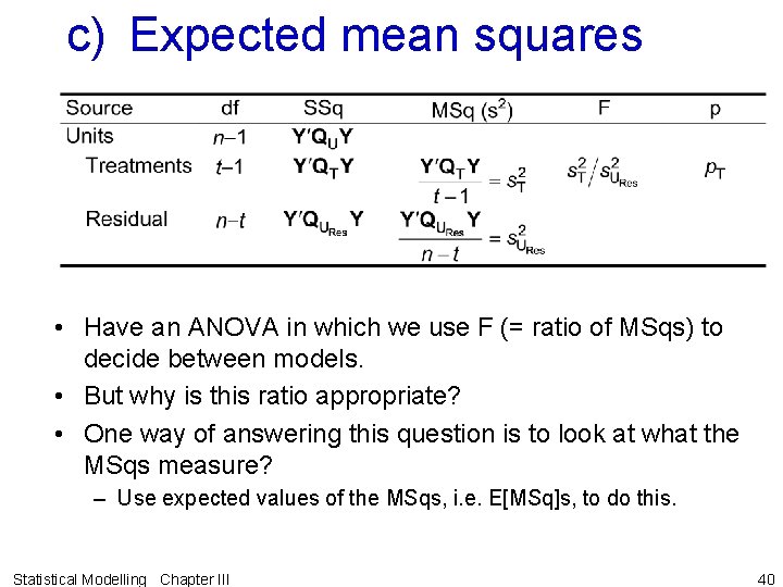
c) Expected mean squares • Have an ANOVA in which we use F (= ratio of MSqs) to decide between models. • But why is this ratio appropriate? • One way of answering this question is to look at what the MSqs measure? – Use expected values of the MSqs, i. e. E[MSq]s, to do this. Statistical Modelling Chapter III 40

Expected mean squares (cont’d) • Remember “expected value = population mean” • Need E[MSq]s – under the maximal model: – and the minimal model: • Similar to asking what is E[Yi]? • Know answer is E[Yi] = ak. – i. e. in population, under model, average value of Yi is ak. • So for Treatments, what is E[MSq]? • The E[MSq]s are the mean values of the MSqs in populations described by the model for which they are derived – i. e. an E[MSq] is the true mean value; – it depends on the model parameters. Statistical Modelling Chapter III 41

E[MSq]s under the maximal model • So if we had the complete populations for all Treatments and computed the MSqs, the value of – the Residual MSq would equal s 2 – the Treatment MSq would equal s 2 + q. T(y). • So that the population average value of both MSqs involves s 2, the uncontrolled variation amongst units from the same treatment. • But what about q in Treatments E[MSq]. Statistical Modelling Chapter III 44

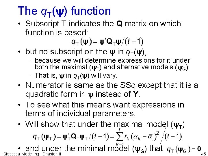
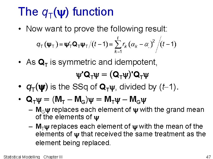
The q. T(y) function • Subscript T indicates the Q matrix on which function is based: • but no subscript on the y in q. T(y), – because we will determine expressions for it under both the maximal (y. T) and alternative models (y. G). – That is, y in q. T(y) will vary. • Numerator is same as the SSq except that it is a quadratic form in y instead of Y. • To see what this means want expressions in terms of individual parameters. • Will show that under the maximal model (y. T) • and under the minimal model (y. G) that Statistical Modelling Chapter III 45

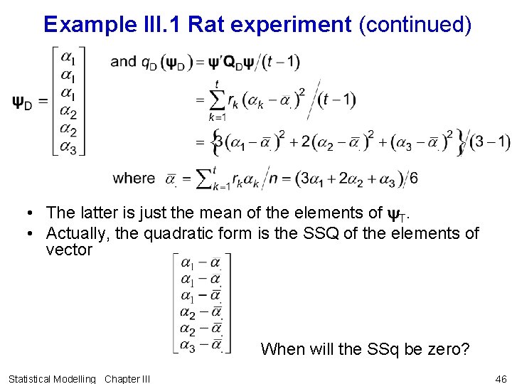
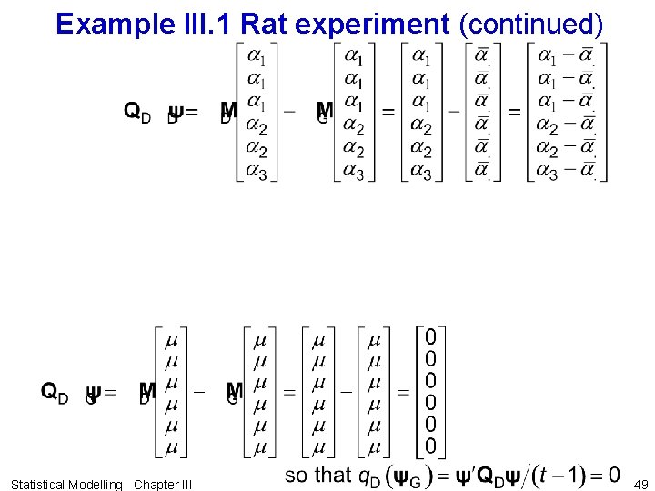
Example III. 1 Rat experiment (continued) • The latter is just the mean of the elements of y. T. • Actually, the quadratic form is the SSQ of the elements of vector When will the SSq be zero? Statistical Modelling Chapter III 46

The q. T(y) function • Now want to prove the following result: • As QT is symmetric and idempotent, y'QTy (QTy)'QTy • q. T(y) is the SSq of QTy, divided by (t-1). • QTy (MT – MG)y MTy – MGy replaces each element of y with the grand mean of the elements of y – MTy replaces each element of y with the mean of the elements of y that received the same treatment as the element being replaced. Statistical Modelling Chapter III 47

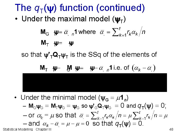
The q. T(y) function (continued) • Under the maximal model (y. T) so that y'TQTy. T is the SSq of the elements of • Under the minimal model (y. G m 1 n) – MGy. G MTy. G so y'GQTy. G 0 and q. T(y) 0; – or ak = m so that – and so that q. T(y) 0. Statistical Modelling Chapter III 48

Example III. 1 Rat experiment (continued) Statistical Modelling Chapter III 49

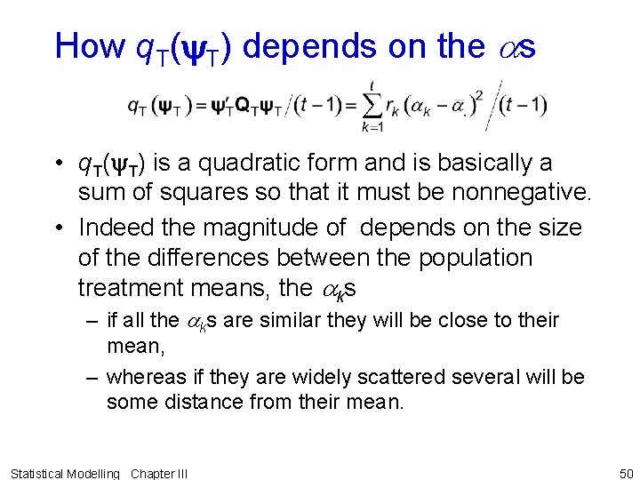
How q. T(y. T) depends on the as • q. T(y. T) is a quadratic form and is basically a sum of squares so that it must be nonnegative. • Indeed the magnitude of depends on the size of the differences between the population treatment means, the aks – if all the aks are similar they will be close to their mean, – whereas if they are widely scattered several will be some distance from their mean. Statistical Modelling Chapter III 50

E[Msq]s in terms of parameters • Could compute population mean of MSq if knew aks and s 2. • Treatment MSq will on average be greater than the Residual MSq – as it is influenced by both uncontrolled variation and the magnitude of treatment differences. • The quadratic form q. T(y) will only be zero when all the as are equal, that is when the null hypothesis is true. – Then the E[MSq]s under the minimal model are equal so that the F value will be approximately one. • Not surprising if think about a particular experiment. Statistical Modelling Chapter III 51

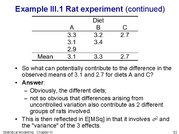
Example III. 1 Rat experiment (continued) • So what can potentially contribute to the difference in the observed means of 3. 1 and 2. 7 for diets A and C? • Answer: – Obviously, the different diets; – not so obvious that differences arising from uncontrolled variation also contribute as 2 different groups of rats involved. • This is then reflected in E[MSq] in that it involves s 2 and the "variance" of the 3 effects. Statistical Modelling Chapter III 52

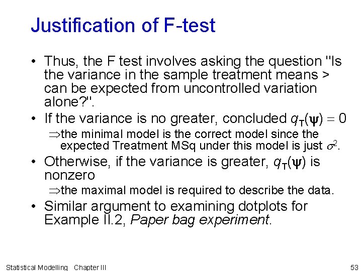
Justification of F-test • Thus, the F test involves asking the question "Is the variance in the sample treatment means > can be expected from uncontrolled variation alone? ". • If the variance is no greater, concluded q. T(y) 0 Þthe minimal model is the correct model since the expected Treatment MSq under this model is just s 2. • Otherwise, if the variance is greater, q. T(y) is nonzero Þthe maximal model is required to describe the data. • Similar argument to examining dotplots for Example II. 2, Paper bag experiment. Statistical Modelling Chapter III 53

d) Summary of the hypothesis test • see notes Statistical Modelling Chapter III 54

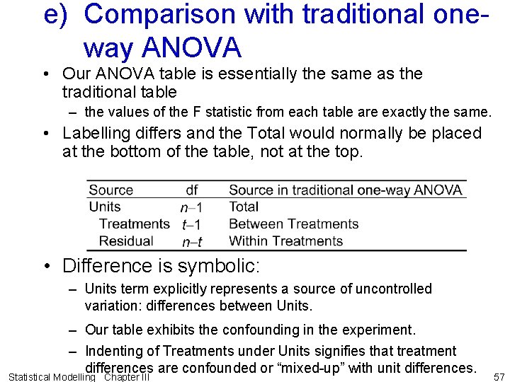
e) Comparison with traditional oneway ANOVA • Our ANOVA table is essentially the same as the traditional table – the values of the F statistic from each table are exactly the same. • Labelling differs and the Total would normally be placed at the bottom of the table, not at the top. • Difference is symbolic: – Units term explicitly represents a source of uncontrolled variation: differences between Units. – Our table exhibits the confounding in the experiment. – Indenting of Treatments under Units signifies that treatment differences are confounded or “mixed-up” with unit differences. Statistical Modelling Chapter III 57

f) Computation of the ANOVA in R • Begin with data entry (see Appendix A, Introduction to R and, Appendix C, Analysis of designed experiments in R) • Next an initial graphical exploration using boxplots — defer to a second example with more data. • ANOVA: while function lm could be used, function aov is preferred for analysing data from a designed experiment. • Both use a model formula of the form: – Response variable ~ explanatory variables (and operators) – So far expressions on right fairly simple — one or two explanatory variables separated by a “+”. • Subtlety with analysis of designed experiments: – If explanatory variable is a numeric, such as a numeric vector, then R fits just one coefficient for it. For a single explanatory variable, a straight-line relationship fitted. – If explanatory variable is categorical, such as a factor, a coefficient is fit for each level of the variable — indicator variables are used. – In analyzing a CRD important that the treatment factor is stored in a factor object, signalling R to use indicator variables Statistical Modelling Chapter III 58

f) Computation of the ANOVA in R (continued) • There are two ways in which this analysis can be obtained using the aov function: – without and with an Error function in the model formula. – Error function used in model formula to specify a model for the Error in the experiment (a model for uncontrolled variation). • summary function is used and this produces ANOVA table. • model. tables function used to obtain tables of means. Statistical Modelling Chapter III 59

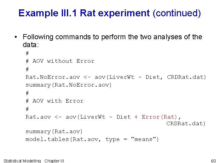
Example III. 1 Rat experiment (continued) • Following commands to perform the two analyses of the data: # # AOV without Error # Rat. No. Error. aov <- aov(Liver. Wt ~ Diet, CRDRat. dat) summary(Rat. No. Error. aov) # # AOV with Error # Rat. aov <- aov(Liver. Wt ~ Diet + Error(Rat), CRDRat. dat) summary(Rat. aov) model. tables(Rat. aov, type = "means") Statistical Modelling Chapter III 60

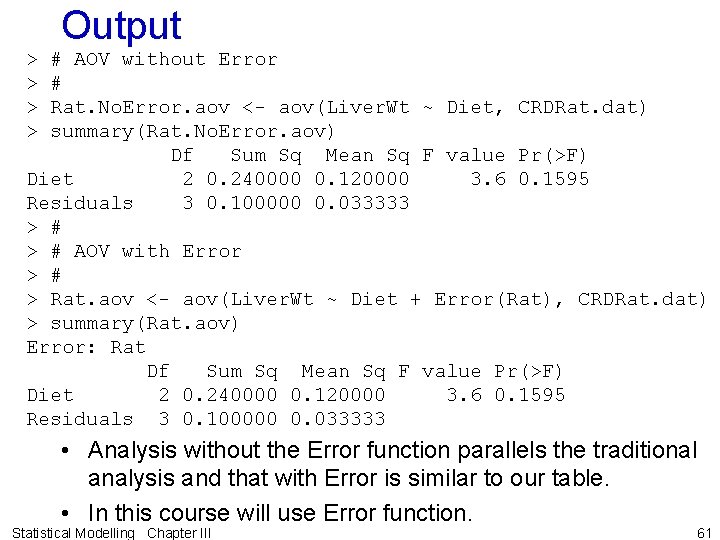
Output > # AOV without Error > # > Rat. No. Error. aov <- aov(Liver. Wt ~ Diet, CRDRat. dat) > summary(Rat. No. Error. aov) Df Sum Sq Mean Sq F value Pr(>F) Diet 2 0. 240000 0. 120000 3. 6 0. 1595 Residuals 3 0. 100000 0. 033333 > # AOV with Error > # > Rat. aov <- aov(Liver. Wt ~ Diet + Error(Rat), CRDRat. dat) > summary(Rat. aov) Error: Rat Df Sum Sq Mean Sq F value Pr(>F) Diet 2 0. 240000 0. 120000 3. 6 0. 1595 Residuals 3 0. 100000 0. 033333 • Analysis without the Error function parallels the traditional analysis and that with Error is similar to our table. • In this course will use Error function. Statistical Modelling Chapter III 61

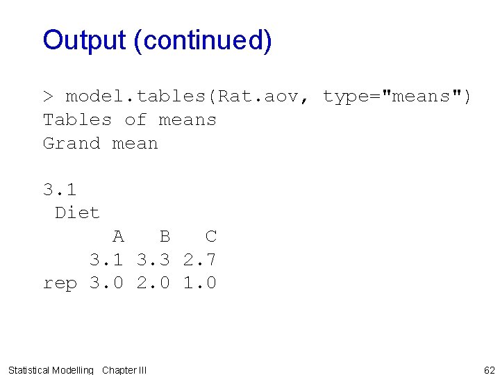
Output (continued) > model. tables(Rat. aov, type="means") Tables of means Grand mean 3. 1 Diet A B C 3. 1 3. 3 2. 7 rep 3. 0 2. 0 1. 0 Statistical Modelling Chapter III 62

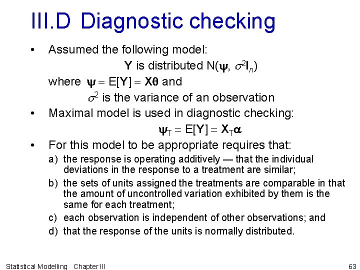
III. D Diagnostic checking • • • Assumed the following model: Y is distributed N(y, s 2 In) where y E[Y] Xq and s 2 is the variance of an observation Maximal model is used in diagnostic checking: y. T E[Y] XTa For this model to be appropriate requires that: a) the response is operating additively — that the individual deviations in the response to a treatment are similar; b) the sets of units assigned the treatments are comparable in that the amount of uncontrolled variation exhibited by them is the same for each treatment; c) each observation is independent of other observations; and d) that the response of the units is normally distributed. Statistical Modelling Chapter III 63

Example III. 2 Caffeine effects on students • Effect of orally ingested caffeine on a physical task was investigated (Draper and Smith, 1981, sec. 9. 1). • Thirty healthy male college students were selected and trained in finger tapping. • Ten men were randomly assigned to receive one of three doses of caffeine (0, 100 or 200 mg). • The number of finger taps after ingesting the caffeine was recorded for each student. Statistical Modelling Chapter III 64

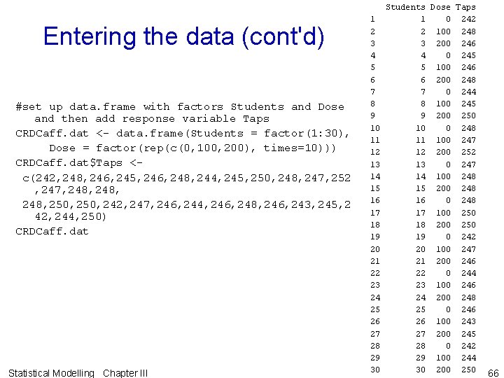
Entering the data • Setting up a data frame, from scratch, for data arranged in standard order (see App C): – factor Students with values 1– 30, – factor Dose with levels 0, 100 and 200 and values depending on whether data is entered by rows or columns (can use rep function), – numeric vector Taps with the 30 observed values of the response variable. Statistical Modelling Chapter III 65

Entering the data (cont'd) #set up data. frame with factors Students and Dose and then add response variable Taps CRDCaff. dat <- data. frame(Students = factor(1: 30), Dose = factor(rep(c(0, 100, 200), times=10))) CRDCaff. dat$Taps <- c(242, 248, 246, 245, 246, 248, 244, 245, 250, 248, 247, 252 , 247, 248, 250, 242, 247, 246, 244, 246, 248, 246, 243, 245, 2 42, 244, 250) CRDCaff. dat Statistical Modelling Chapter III Students Dose Taps 1 0 242 2 2 100 248 3 3 200 246 4 0 245 5 5 100 246 6 6 200 248 7 0 244 8 8 100 245 9 9 200 250 10 0 248 11 100 247 12 200 252 13 0 247 14 100 248 15 200 248 16 0 248 17 100 250 18 200 250 19 0 242 20 100 247 21 200 246 22 0 244 23 100 246 24 200 248 25 0 246 26 100 243 27 200 245 28 0 242 29 100 244 30 200 250 66

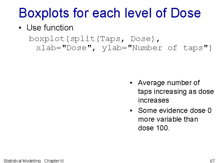
Boxplots for each level of Dose • Use function boxplot(split(Taps, Dose), xlab="Dose", ylab="Number of taps") • Average number of taps increasing as dose increases • Some evidence dose 0 more variable than dose 100. Statistical Modelling Chapter III 67

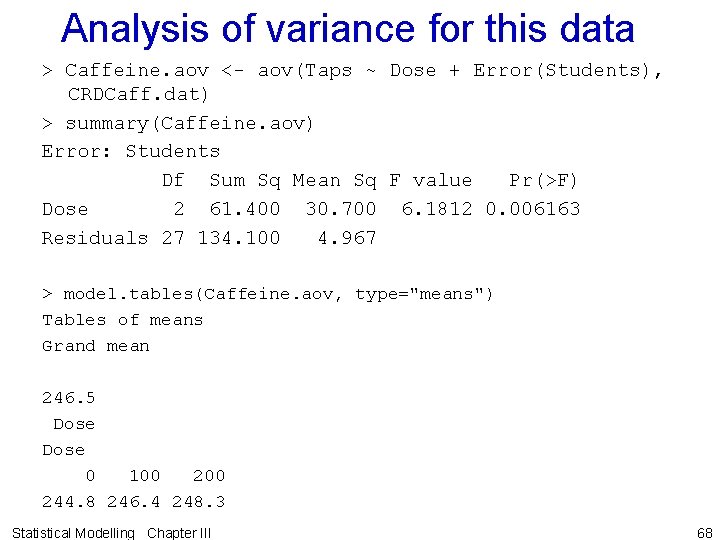
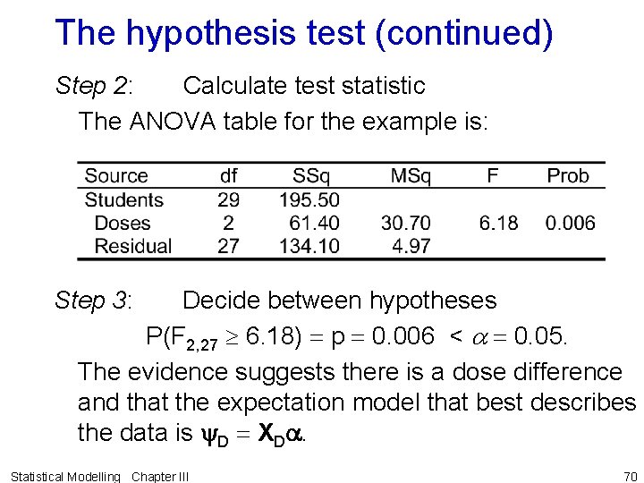
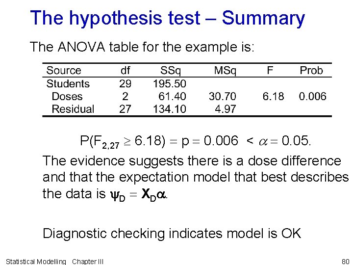
Analysis of variance for this data > Caffeine. aov <- aov(Taps ~ Dose + Error(Students), CRDCaff. dat) > summary(Caffeine. aov) Error: Students Df Sum Sq Mean Sq F value Pr(>F) Dose 2 61. 400 30. 700 6. 1812 0. 006163 Residuals 27 134. 100 4. 967 > model. tables(Caffeine. aov, type="means") Tables of means Grand mean 246. 5 Dose 0 100 200 244. 8 246. 4 248. 3 Statistical Modelling Chapter III 68

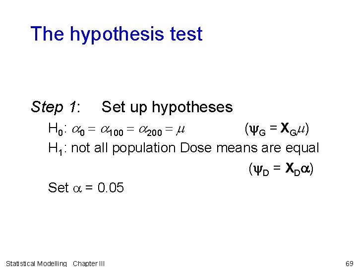
The hypothesis test Step 1: Set up hypotheses H 0: a 0 a 100 a 200 m (y. G = XGm) H 1: not all population Dose means are equal (y. D = XDa) Set a = 0. 05 Statistical Modelling Chapter III 69

The hypothesis test (continued) Step 2: Calculate test statistic The ANOVA table for the example is: Step 3: Decide between hypotheses P(F 2, 27 6. 18) p 0. 006 < a 0. 05. The evidence suggests there is a dose difference and that the expectation model that best describes the data is y. D XDa. Statistical Modelling Chapter III 70

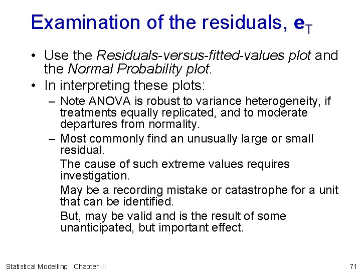
Examination of the residuals, e. T • Use the Residuals-versus-fitted-values plot and the Normal Probability plot. • In interpreting these plots: – Note ANOVA is robust to variance heterogeneity, if treatments equally replicated, and to moderate departures from normality. – Most commonly find an unusually large or small residual. The cause of such extreme values requires investigation. May be a recording mistake or catastrophe for a unit that can be identified. But, may be valid and is the result of some unanticipated, but important effect. Statistical Modelling Chapter III 71

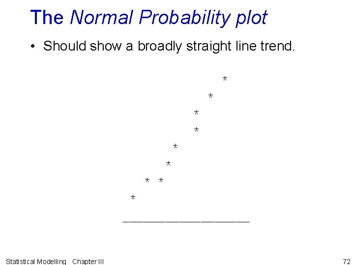
The Normal Probability plot • Should show a broadly straight line trend. * * * * * _________ Statistical Modelling Chapter III 72

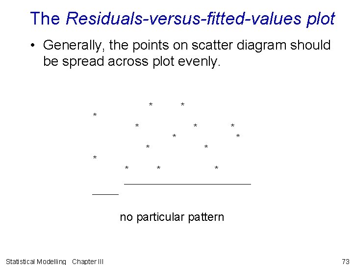
The Residuals-versus-fitted-values plot • Generally, the points on scatter diagram should be spread across plot evenly. * * * * * * * * * * ____________ no particular pattern Statistical Modelling Chapter III 73

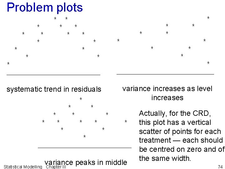
Problem plots * * * * * * * _____________ * * * * * _____________ systematic trend in residuals variance increases as level increases * * * * * * _____________ variance peaks in middle Statistical Modelling Chapter III Actually, for the CRD, this plot has a vertical scatter of points for each treatment — each should be centred on zero and of the same width. 74

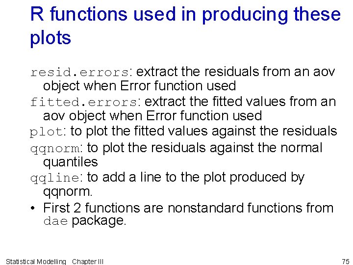
R functions used in producing these plots resid. errors: extract the residuals from an aov object when Error function used fitted. errors: extract the fitted values from an aov object when Error function used plot: to plot the fitted values against the residuals qqnorm: to plot the residuals against the normal quantiles qqline: to add a line to the plot produced by qqnorm. • First 2 functions are nonstandard functions from dae package. Statistical Modelling Chapter III 75

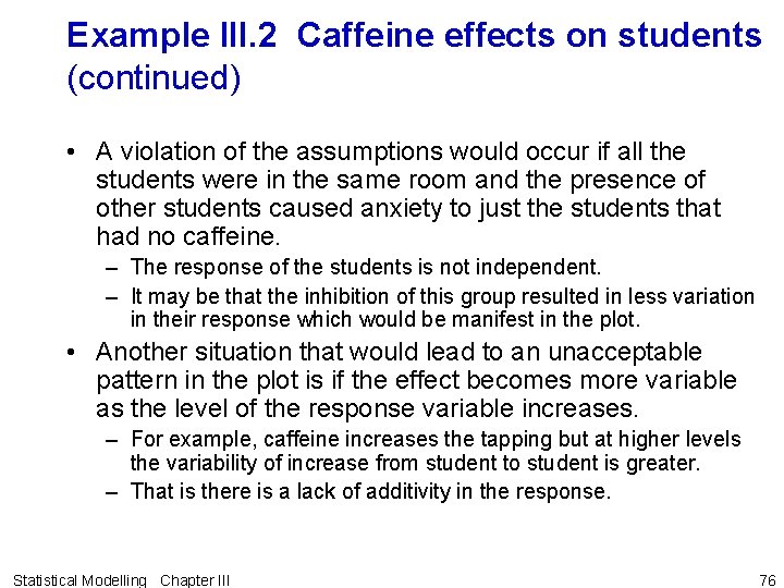
Example III. 2 Caffeine effects on students (continued) • A violation of the assumptions would occur if all the students were in the same room and the presence of other students caused anxiety to just the students that had no caffeine. – The response of the students is not independent. – It may be that the inhibition of this group resulted in less variation in their response which would be manifest in the plot. • Another situation that would lead to an unacceptable pattern in the plot is if the effect becomes more variable as the level of the response variable increases. – For example, caffeine increases the tapping but at higher levels the variability of increase from student to student is greater. – That is there is a lack of additivity in the response. Statistical Modelling Chapter III 76

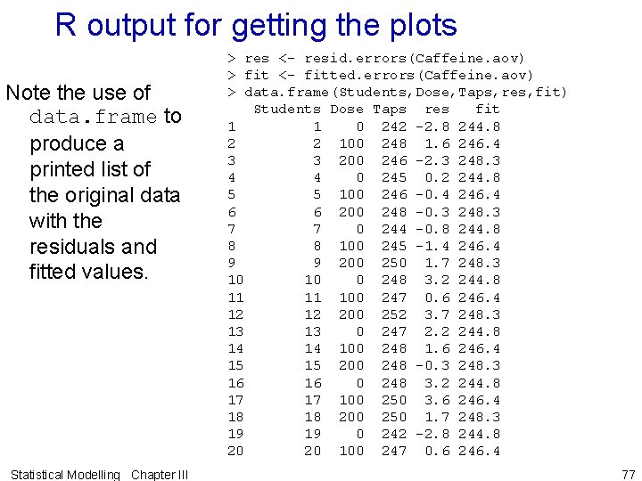
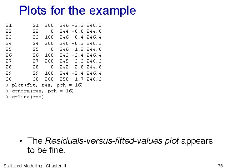
R output for getting the plots Note the use of data. frame to produce a printed list of the original data with the residuals and fitted values. Statistical Modelling Chapter III > res <- resid. errors(Caffeine. aov) > fit <- fitted. errors(Caffeine. aov) > data. frame(Students, Dose, Taps, res, fit) Students Dose Taps res fit 1 0 242 -2. 8 244. 8 2 2 100 248 1. 6 246. 4 3 3 200 246 -2. 3 248. 3 4 0 245 0. 2 244. 8 5 5 100 246 -0. 4 246. 4 6 6 200 248 -0. 3 248. 3 7 0 244 -0. 8 244. 8 8 8 100 245 -1. 4 246. 4 9 9 200 250 1. 7 248. 3 10 0 248 3. 2 244. 8 11 100 247 0. 6 246. 4 12 200 252 3. 7 248. 3 13 0 247 2. 2 244. 8 14 100 248 1. 6 246. 4 15 200 248 -0. 3 248. 3 16 0 248 3. 2 244. 8 17 100 250 3. 6 246. 4 18 200 250 1. 7 248. 3 19 0 242 -2. 8 244. 8 20 100 247 0. 6 246. 4 77

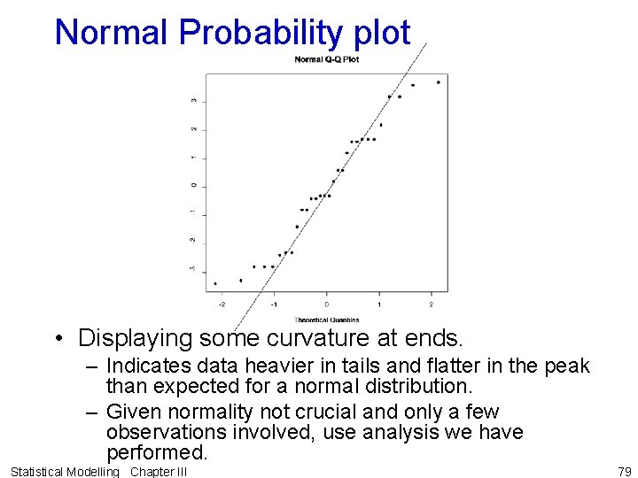
Plots for the example 21 200 246 -2. 3 248. 3 22 0 244 -0. 8 244. 8 23 100 246 -0. 4 246. 4 24 200 248 -0. 3 248. 3 25 0 246 1. 2 244. 8 26 100 243 -3. 4 246. 4 27 200 245 -3. 3 248. 3 28 0 242 -2. 8 244. 8 29 100 244 -2. 4 246. 4 30 200 250 1. 7 248. 3 > plot(fit, res, pch = 16) > qqnorm(res, pch = 16) > qqline(res) • The Residuals-versus-fitted-values plot appears to be fine. Statistical Modelling Chapter III 78

Normal Probability plot • Displaying some curvature at ends. – Indicates data heavier in tails and flatter in the peak than expected for a normal distribution. – Given normality not crucial and only a few observations involved, use analysis we have performed. Statistical Modelling Chapter III 79

The hypothesis test – Summary The ANOVA table for the example is: P(F 2, 27 6. 18) p 0. 006 < a 0. 05. The evidence suggests there is a dose difference and that the expectation model that best describes the data is y. D XDa. Diagnostic checking indicates model is OK Statistical Modelling Chapter III 80

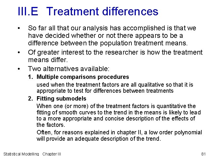
III. E Treatment differences • • • So far all that our analysis has accomplished is that we have decided whether or not there appears to be a difference between the population treatment means. Of greater interest to the researcher is how the treatment means differ. Two alternatives available: 1. Multiple comparisons procedures used when the treatment factors are all qualitative so that it is appropriate to test for differences between treatments 2. Fitting submodels When one (or more) of the treatment factors is quantitative the fitting of smooth curves to the trend in the means is likely to lead to a more appropriate and concise description of the effects of the factors. Often, for reasons explained in chapter II, a low order polynomial will provide an adequate description of the trend. Statistical Modelling Chapter III 81

Note • Multiple comparison procedures should not be used when the test for treatment differences is not significant. • Submodels should be fitted irrespective of whether the overall test for treatment differences is significant. • The difference in usage has to do with one being concerned with mean differences and the other with deciding between models. Statistical Modelling Chapter III 82

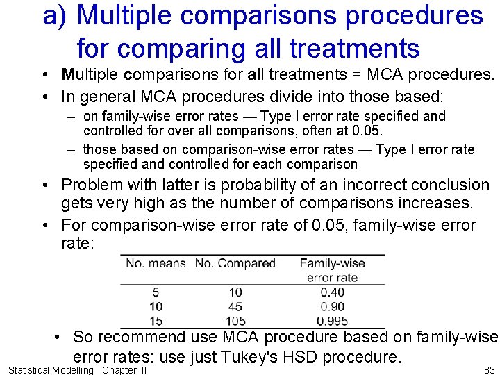
a) Multiple comparisons procedures for comparing all treatments • Multiple comparisons for all treatments = MCA procedures. • In general MCA procedures divide into those based: – on family-wise error rates — Type I error rate specified and controlled for over all comparisons, often at 0. 05. – those based on comparison-wise error rates — Type I error rate specified and controlled for each comparison • Problem with latter is probability of an incorrect conclusion gets very high as the number of comparisons increases. • For comparison-wise error rate of 0. 05, family-wise error rate: • So recommend use MCA procedure based on family-wise error rates: use just Tukey's HSD procedure. Statistical Modelling Chapter III 83

Tukey’s Honestly Significant Difference procedure • determines if each pair of means is significantly different • is based on a family-wise error rate. • basically for equal numbers of observations for each mean. A modification that is approximate will be provided for unequal numbers. Statistical Modelling Chapter III 84

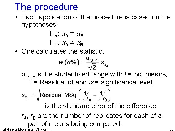
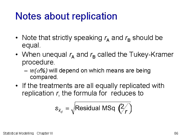
The procedure • Each application of the procedure is based on the hypotheses: Ho: a. A = a. B H 1: a. A a. B • One calculates the statistic: qt, n, a is the studentized range with t = no. means, n = Residual df and a = significance level, is the standard error of the difference r. A, r. B are the number of replicates for each of a pair of means being compared. Statistical Modelling Chapter III 85

Notes about replication • Note that strictly speaking r. A and r. B should be equal. • When unequal r. A and r. B called the Tukey-Kramer procedure. – w(a%) will depend on which means are being compared. • If the treatments are all equally replicated with replication r, the formula for reduces to Statistical Modelling Chapter III 86

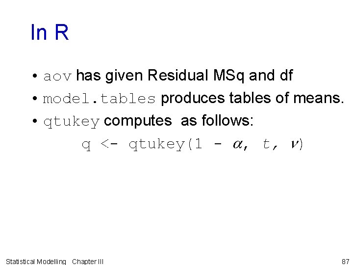
In R • aov has given Residual MSq and df • model. tables produces tables of means. • qtukey computes as follows: q <- qtukey(1 - a, t, n) Statistical Modelling Chapter III 87

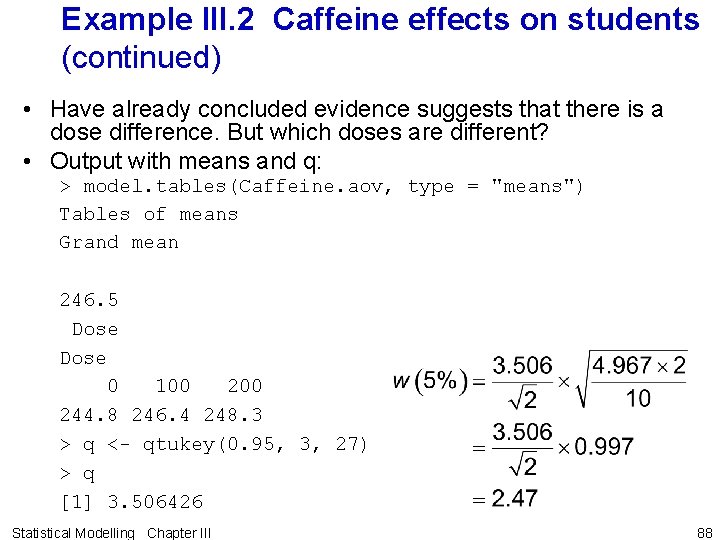
Example III. 2 Caffeine effects on students (continued) • Have already concluded evidence suggests that there is a dose difference. But which doses are different? • Output with means and q: > model. tables(Caffeine. aov, type = "means") Tables of means Grand mean 246. 5 Dose 0 100 200 244. 8 246. 4 248. 3 > q <- qtukey(0. 95, 3, 27) > q [1] 3. 506426 Statistical Modelling Chapter III 88

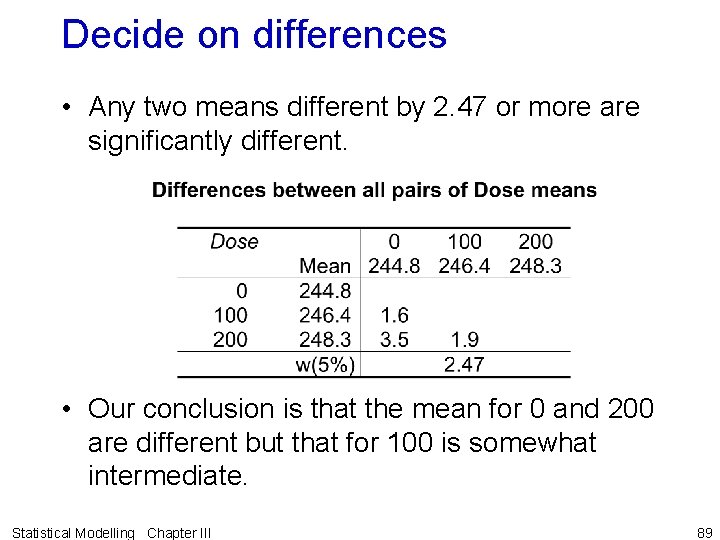
Decide on differences • Any two means different by 2. 47 or more are significantly different. • Our conclusion is that the mean for 0 and 200 are different but that for 100 is somewhat intermediate. Statistical Modelling Chapter III 89

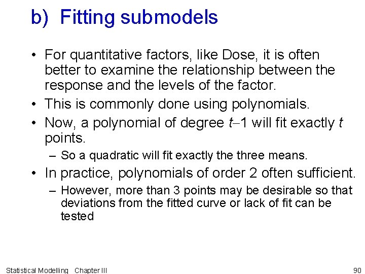
b) Fitting submodels • For quantitative factors, like Dose, it is often better to examine the relationship between the response and the levels of the factor. • This is commonly done using polynomials. • Now, a polynomial of degree t-1 will fit exactly t points. – So a quadratic will fit exactly the three means. • In practice, polynomials of order 2 often sufficient. – However, more than 3 points may be desirable so that deviations from the fitted curve or lack of fit can be tested Statistical Modelling Chapter III 90

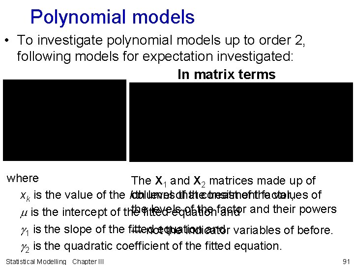
Polynomial models • To investigate polynomial models up to order 2, following models for expectation investigated: In matrix terms where The X 1 and X 2 matrices made up of columns that consist of the values of xk is the value of the kth level of the treatment factor, the levels of the factor and their powers m is the intercept of the fitted equation and g 1 is the slope of the fitted equation and — not the indicator variables of before. g 2 is the quadratic coefficient of the fitted equation. Statistical Modelling Chapter III 91

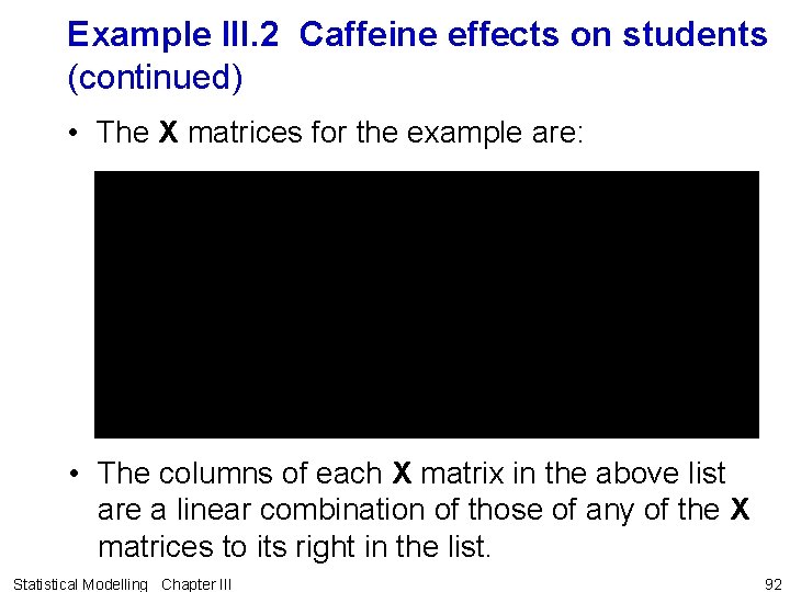
Example III. 2 Caffeine effects on students (continued) • The X matrices for the example are: • The columns of each X matrix in the above list are a linear combination of those of any of the X matrices to its right in the list. Statistical Modelling Chapter III 92

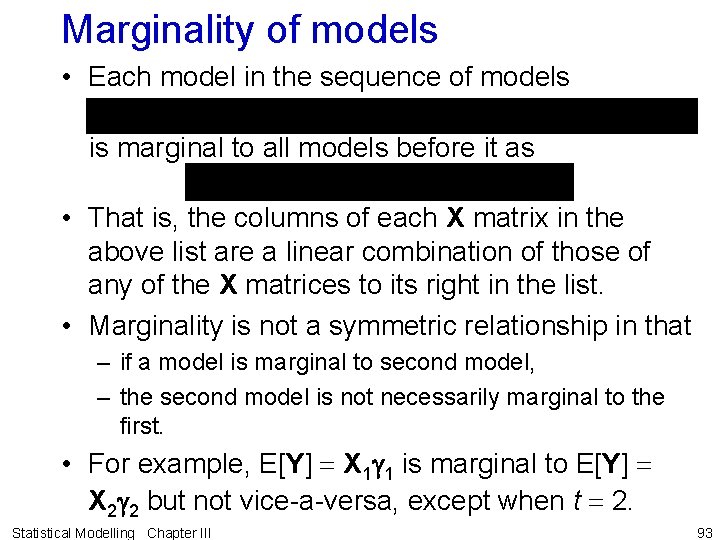
Marginality of models • Each model in the sequence of models is marginal to all models before it as • That is, the columns of each X matrix in the above list are a linear combination of those of any of the X matrices to its right in the list. • Marginality is not a symmetric relationship in that – if a model is marginal to second model, – the second model is not necessarily marginal to the first. • For example, E[Y] X 1 g 1 is marginal to E[Y] X 2 g 2 but not vice-a-versa, except when t 2. Statistical Modelling Chapter III 93

Equivalence of E[Y] X 2 g 2 and E[Y] XDa • C(X 2) C(XD) as the 3 columns of one matrix can be written as 3 linearly independent combinations of the columns of the other matrix. • So the two models are marginal to each other and are equivalent • However, while the fitted values are the same, the estimates and interpretation of the parameters are different: – those corresponding to X 2 are interpreted as the intercept, slope and curvature coefficient. – those corresponding to XD are interpreted as the expected (mean) value for that treatment. • Also, in spite of being marginal, the estimators of the same parameter differ depending on the model that has been fitted. – for example, for the model E[Y] XGm, models not – but for E[Y] X 1 g 1, orthogonal Statistical Modelling Chapter III 94

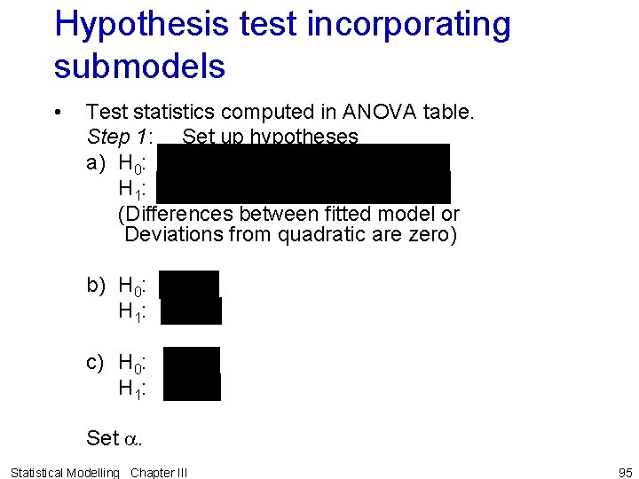
Hypothesis test incorporating submodels • Test statistics computed in ANOVA table. Step 1: Set up hypotheses a) H 0: H 1: (Differences between fitted model or Deviations from quadratic are zero) b) H 0: H 1: c) H 0: H 1: Set a. Statistical Modelling Chapter III 95

Hypothesis test (continued) Step 2: Calculate test statistics The ANOVA table for a CRD is: Test statistics corresponds to hypothesis pairs in Step 1. Statistical Modelling Chapter III 96

Hypothesis test (continued) Step 3: Decide between hypotheses Begin with the first hypothesis pair, determine its significance and continue down the sequence until a significant result is obtained. – A significant Deviations F indicates that the linear and quadratic terms provide an inadequate description. Thus a model based on them would be unsatisfactory. No point in continuing. – If the Deviations F is not significant , then a significant Quadratic F indicates that a 2 nd degree polynomial is required to adequately describe the trend. As a linear coefficient is necessarily incorporated in a 2 nd polynomial, no point to further testing in this case. – If both the Deviations and Quadratic F's are not significant, then a significant Linear F indicates a linear relationship describes the trend in the treatment means. Statistical Modelling Chapter III 97

What if deviations is significant? • If the Deviations are significant, then two options are: a) increase the degree of the polynomial (often not desirable), or b) use multiple comparisons to investigate the differences between the means. Statistical Modelling Chapter III 98

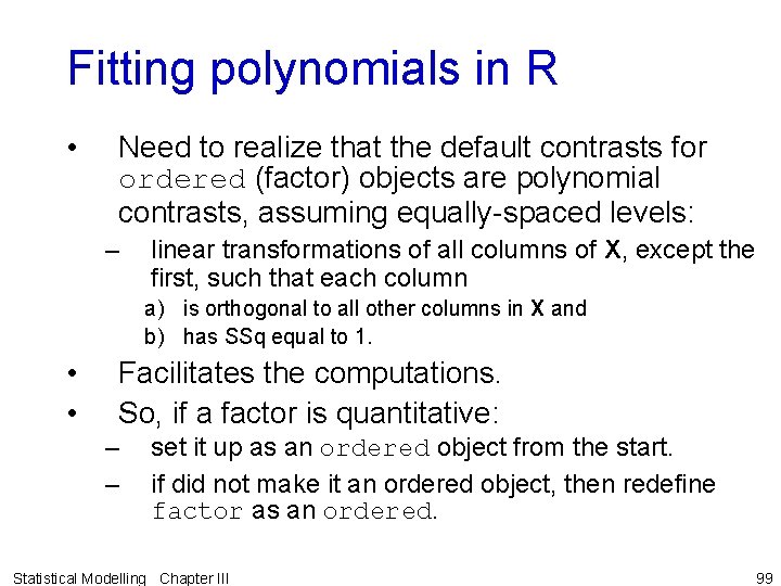
Fitting polynomials in R • Need to realize that the default contrasts for ordered (factor) objects are polynomial contrasts, assuming equally-spaced levels: – linear transformations of all columns of X, except the first, such that each column a) is orthogonal to all other columns in X and b) has SSq equal to 1. • • Facilitates the computations. So, if a factor is quantitative: – – set it up as an ordered object from the start. if did not make it an ordered object, then redefine factor as an ordered. Statistical Modelling Chapter III 99

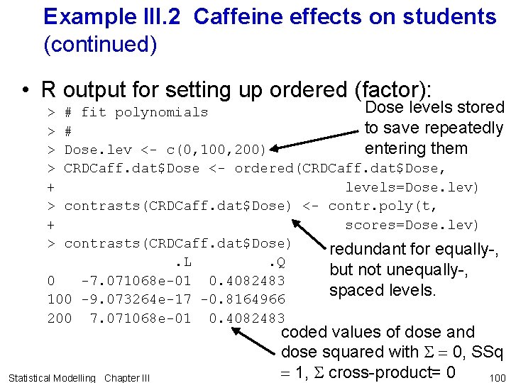
Example III. 2 Caffeine effects on students (continued) • R output for setting up ordered (factor): Dose levels stored > # fit polynomials to save repeatedly > # entering them > Dose. lev <- c(0, 100, 200) > CRDCaff. dat$Dose <- ordered(CRDCaff. dat$Dose, + levels=Dose. lev) > contrasts(CRDCaff. dat$Dose) <- contr. poly(t, + scores=Dose. lev) > contrasts(CRDCaff. dat$Dose) redundant for equally-, . L . Q but not unequally-, 0 -7. 071068 e-01 0. 4082483 spaced levels. 100 -9. 073264 e-17 -0. 8164966 200 7. 071068 e-01 0. 4082483 Statistical Modelling Chapter III coded values of dose and dose squared with S 0, SSq 1, S cross-product= 0 100

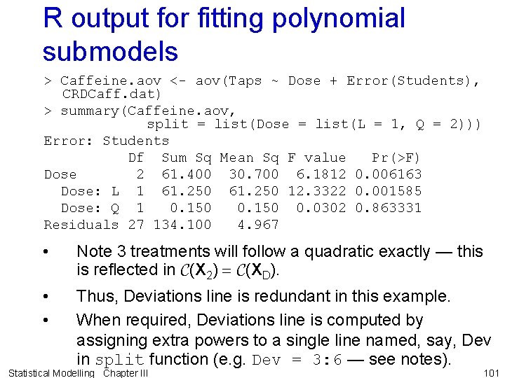
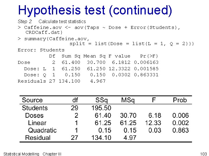
R output for fitting polynomial submodels > Caffeine. aov <- aov(Taps ~ Dose + Error(Students), CRDCaff. dat) > summary(Caffeine. aov, split = list(Dose = list(L = 1, Q = 2))) Error: Students Df Sum Sq Mean Sq F value Pr(>F) Dose 2 61. 400 30. 700 6. 1812 0. 006163 Dose: L 1 61. 250 12. 3322 0. 001585 Dose: Q 1 0. 150 0. 0302 0. 863331 Residuals 27 134. 100 4. 967 • Note 3 treatments will follow a quadratic exactly — this is reflected in C(X 2) C(XD). • • Thus, Deviations line is redundant in this example. When required, Deviations line is computed by assigning extra powers to a single line named, say, Dev in split function (e. g. Dev = 3: 6 — see notes). Statistical Modelling Chapter III 101

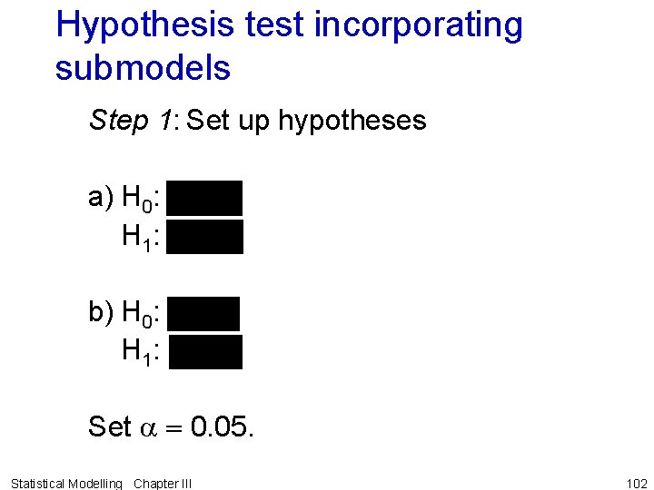
Hypothesis test incorporating submodels Step 1: Set up hypotheses a) H 0: H 1: b) H 0: H 1: Set a 0. 05. Statistical Modelling Chapter III 102

Hypothesis test (continued) Step 2: Calculate test statistics > Caffeine. aov <- aov(Taps ~ Dose + Error(Students), CRDCaff. dat) > summary(Caffeine. aov, split = list(Dose = list(L = 1, Q = 2))) Error: Students Df Sum Sq Mean Sq F value Pr(>F) Dose 2 61. 400 30. 700 6. 1812 0. 006163 Dose: L 1 61. 250 12. 3322 0. 001585 Dose: Q 1 0. 150 0. 0302 0. 863331 Residuals 27 134. 100 4. 967 Statistical Modelling Chapter III 103

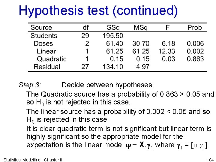
Hypothesis test (continued) Step 3: Decide between hypotheses The Quadratic source has a probability of 0. 863 > 0. 05 and so H 0 is not rejected in this case. The linear source has a probability of 0. 002 < 0. 05 and so H 0 is rejected in this case. It is clear quadratic term is not significant but linear term is highly significant so the appropriate model for the expectation is the linear model y X 1 g 1 where g 1 = [m g 1]. Statistical Modelling Chapter III 104

Fitted equation • Coefficients can be obtained using the coef function on the aov object, but these are not suitable for obtaining the fitted values. • The fitted equation is obtained by putting the values of the levels into a numeric vector and using the lm function to fit a polynomial of the order indicated by the hypothesis test. • For the example, linear equation was adequate and so the analysis is redone with 1 for the order of the polynomial. Statistical Modelling Chapter III 105

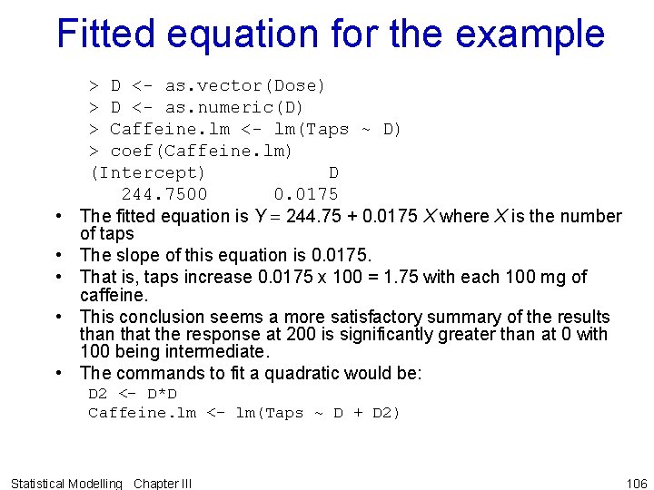
Fitted equation for the example • • • > D <- as. vector(Dose) > D <- as. numeric(D) > Caffeine. lm <- lm(Taps ~ D) > coef(Caffeine. lm) (Intercept) D 244. 7500 0. 0175 The fitted equation is Y 244. 75 + 0. 0175 X where X is the number of taps The slope of this equation is 0. 0175. That is, taps increase 0. 0175 x 100 = 1. 75 with each 100 mg of caffeine. This conclusion seems a more satisfactory summary of the results than that the response at 200 is significantly greater than at 0 with 100 being intermediate. The commands to fit a quadratic would be: D 2 <- D*D Caffeine. lm <- lm(Taps ~ D + D 2) Statistical Modelling Chapter III 106

Plotting means and fitted line • Details are in the notes • The plot produced is as follows: Statistical Modelling Chapter III 107

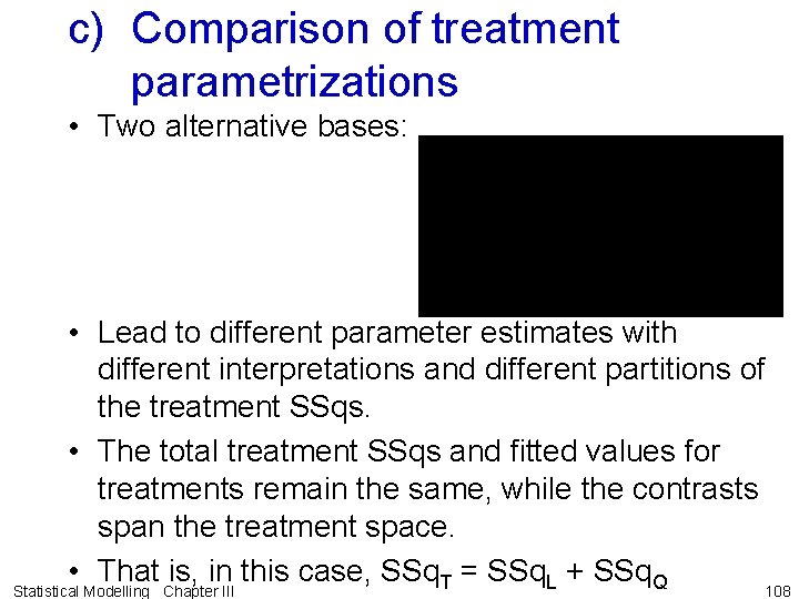
c) Comparison of treatment parametrizations • Two alternative bases: • Lead to different parameter estimates with different interpretations and different partitions of the treatment SSqs. • The total treatment SSqs and fitted values for treatments remain the same, while the contrasts span the treatment space. • That is, in this case, SSq. T = SSq. L + SSq. Q 108 Statistical Modelling Chapter III

III. G Exercises • Ex. III. 1– 2 look at aspects of quadratic forms • Ex. III. 3 investigates the calculations with example that can be done with a calculator • Ex. III. 4 involves producing a randomized layout • Ex. III. 5 asks for the complete analysis of a CRD with a qualitative treatment factor • Ex. III. 6 asks for the complete analysis of a CRD with a quantitative treatment factor Statistical Modelling Chapter III 109