Radiative transfer in numerical models of the atmosphere

Radiative transfer in numerical models of the atmosphere Robin Hogan Slides contain contributions from Jean-Jacques Morcrette, Alessio Bozzo, Tony Slingo and Piers Forster

Outline • Lectures 1 & 2 1. Global context 2. From Maxwell to the two-stream equations 3. Gaseous absorption and emission • Lecture 3 (Alessio Bozzo) – The ECMWF radiation scheme • Lecture 4 4. Representing cloud structure 5. Some remaining challenges

Part 4: Representing cloud structure • Representing cloud fraction, overlap and inhomogeneity • What is the impact of overlap and inhomogeneity on the radiation budget?

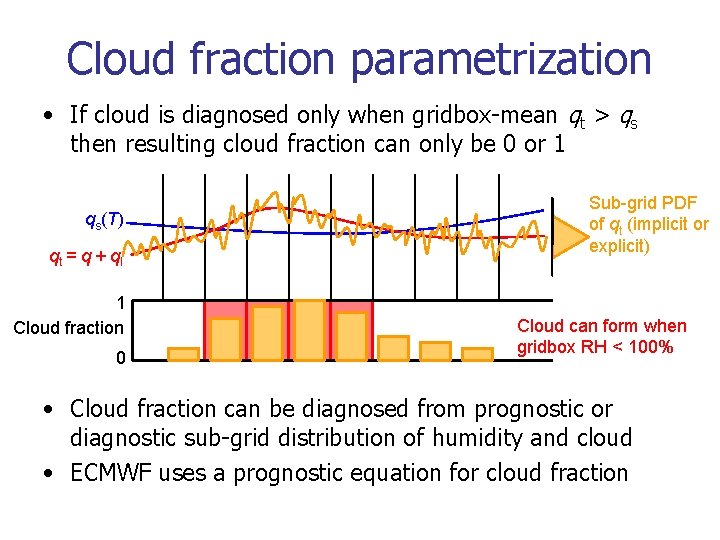
Cloud fraction parametrization • If cloud is diagnosed only when gridbox-mean qt > qs then resulting cloud fraction can only be 0 or 1 qs(T) qt = q + ql 1 Cloud fraction 0 Sub-grid PDF of qt (implicit or explicit) Cloud can form when gridbox RH < 100% • Cloud fraction can be diagnosed from prognostic or diagnostic sub-grid distribution of humidity and cloud • ECMWF uses a prognostic equation for cloud fraction

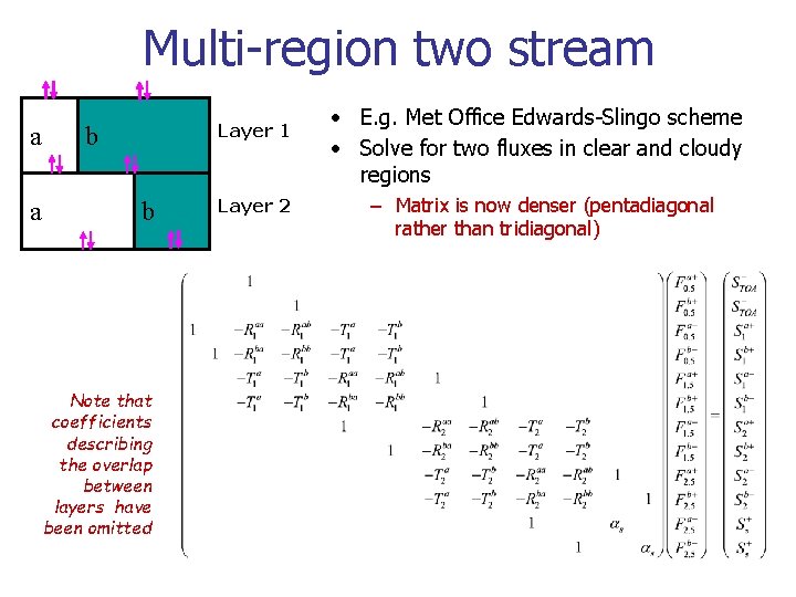
Multi-region two stream a a Layer 1 b b Note that coefficients describing the overlap between layers have been omitted Layer 2 • E. g. Met Office Edwards-Slingo scheme • Solve for two fluxes in clear and cloudy regions – Matrix is now denser (pentadiagonal rather than tridiagonal)

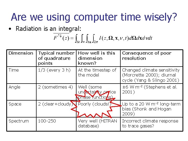
Are we using computer time wisely? • Radiation is an integral: Dimension Typical number How well is this of quadrature dimension points known? Consequence of poor resolution Time 1/3 (every 3 h) At the timestep of the model Changed climate sensitivity (Morcrette 2000); diurnal cycle (Yang & Slingo 2001) Angle 2 (sometimes 4) Well (some uncertainty on ice phase functions) ± 6 W m-2 (Stephens et al. 2001) Space 2 (clear+cloudy) Poorly (clouds!) Up to a 20 W m-2 long-term bias (Shonk and Hogan 2009) Spectrum 100 -250 Very well (HITRAN database) Incorrect climate response to trace gases?

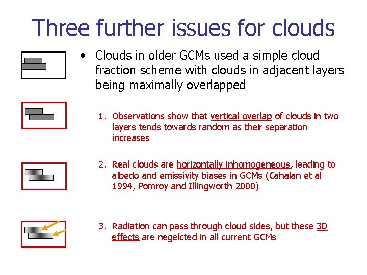
Three further issues for clouds • Clouds in older GCMs used a simple cloud fraction scheme with clouds in adjacent layers being maximally overlapped 1. Observations show that vertical overlap of clouds in two layers tends towards random as their separation increases 2. Real clouds are horizontally inhomogeneous, leading to albedo and emissivity biases in GCMs (Cahalan et al 1994, Pomroy and Illingworth 2000) 3. Radiation can pass through cloud sides, but these 3 D effects are negelcted in all current GCMs

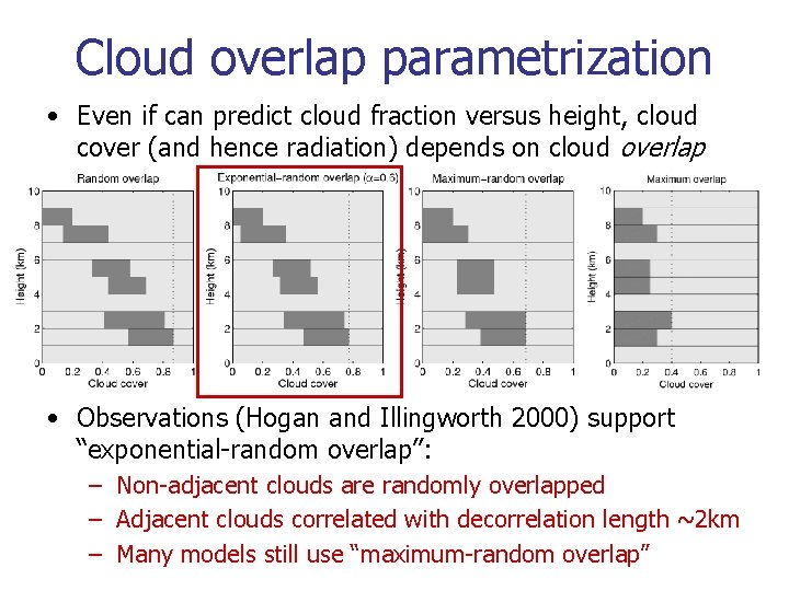
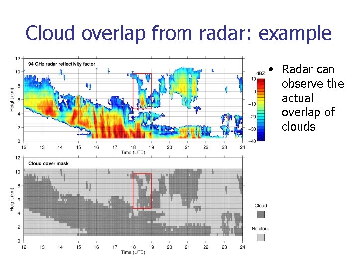
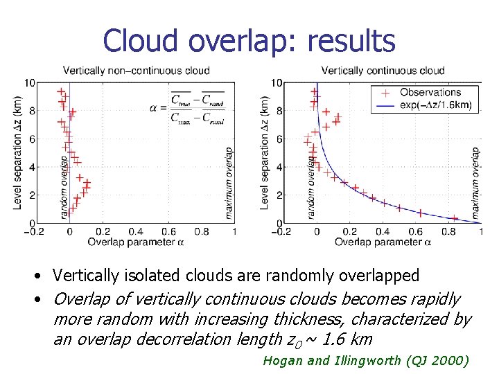
Cloud overlap parametrization • Even if can predict cloud fraction versus height, cloud cover (and hence radiation) depends on cloud overlap – sdfsdfs • Observations (Hogan and Illingworth 2000) support “exponential-random overlap”: − Non-adjacent clouds are randomly overlapped − Adjacent clouds correlated with decorrelation length ~2 km − Many models still use “maximum-random overlap”

Cloud overlap from radar: example • Radar can observe the actual overlap of clouds

Cloud overlap: results • Vertically isolated clouds are randomly overlapped • Overlap of vertically continuous clouds becomes rapidly more random with increasing thickness, characterized by an overlap decorrelation length z 0 ~ 1. 6 km Hogan and Illingworth (QJ 2000)

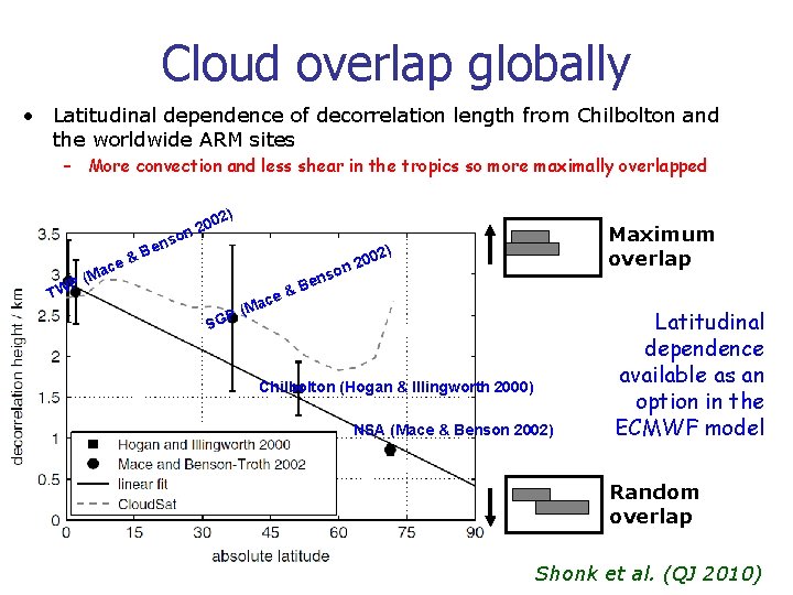
Cloud overlap globally • Latitudinal dependence of decorrelation length from Chilbolton and the worldwide ARM sites – More convection and less shear in the tropics so more maximally overlapped ) 002 2 n P TW ce (Ma & nso Be P (M G S ace on ens 20 Maximum overlap 02) &B Chilbolton (Hogan & Illingworth 2000) NSA (Mace & Benson 2002) Latitudinal dependence available as an option in the ECMWF model Random overlap Shonk et al. (QJ 2010)

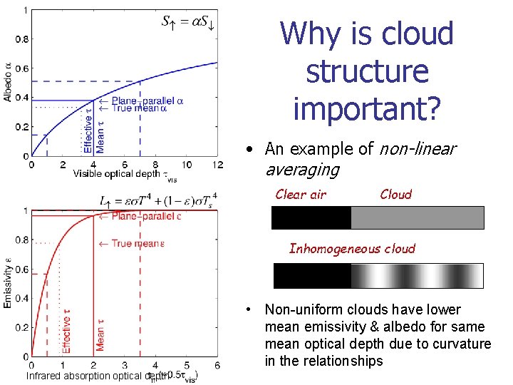
Why is cloud structure important? • An example of non-linear averaging Clear air Cloud Inhomogeneous cloud • Non-uniform clouds have lower mean emissivity & albedo for same mean optical depth due to curvature in the relationships Infrared absorption optical depth

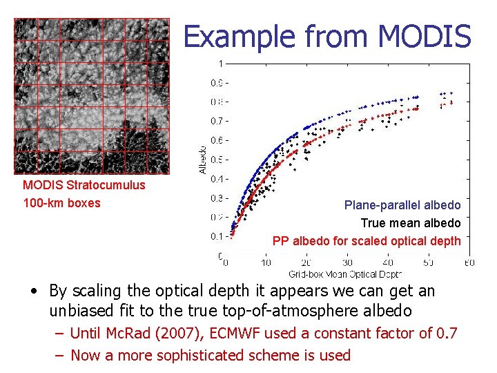
Example from MODIS Stratocumulus 100 -km boxes Plane-parallel albedo True mean albedo PP albedo for scaled optical depth • By scaling the optical depth it appears we can get an unbiased fit to the true top-of-atmosphere albedo – Until Mc. Rad (2007), ECMWF used a constant factor of 0. 7 – Now a more sophisticated scheme is used

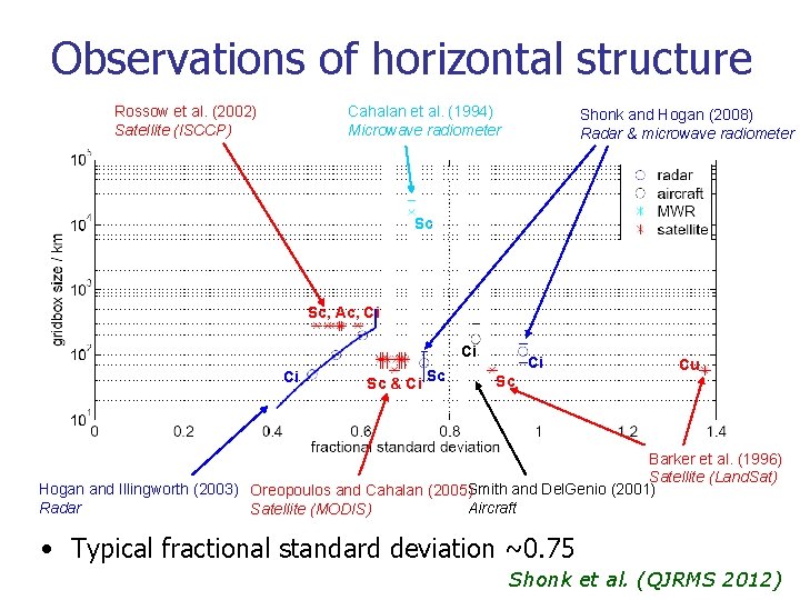
Observations of horizontal structure Rossow et al. (2002) Satellite (ISCCP) Cahalan et al. (1994) Microwave radiometer Shonk and Hogan (2008) Radar & microwave radiometer Sc Sc, Ac, Ci Ci Ci Sc & Ci Sc Ci Cu Sc Barker et al. (1996) Satellite (Land. Sat) Hogan and Illingworth (2003) Oreopoulos and Cahalan (2005)Smith and Del. Genio (2001) Radar Aircraft Satellite (MODIS) • Typical fractional standard deviation ~0. 75 Shonk et al. (QJRMS 2012)

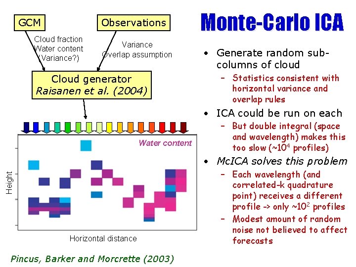
GCM Observations Cloud fraction Water content (Variance? ) Variance Overlap assumption Cloud generator Raisanen et al. (2004) Monte-Carlo ICA • Generate random subcolumns of cloud – Statistics consistent with horizontal variance and overlap rules • ICA could be run on each Water content – But double integral (space and wavelength) makes this too slow (~104 profiles) Height • Mc. ICA solves this problem Horizontal distance Pincus, Barker and Morcrette (2003) – Each wavelength (and correlated-k quadrature point) receives a different profile -> only ~102 profiles – Modest amount of random noise not believed to affect forecasts

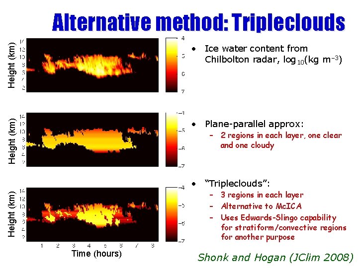
Height (km) • Ice water content from Chilbolton radar, log 10(kg m– 3) Height (km) Alternative method: Tripleclouds • Plane-parallel approx: – 2 regions in each layer, one clear and one cloudy • “Tripleclouds”: Height (km) – 3 regions in each layer – Alternative to Mc. ICA – Uses Edwards-Slingo capability for stratiform/convective regions for another purpose Time (hours) Shonk and Hogan (JClim 2008)

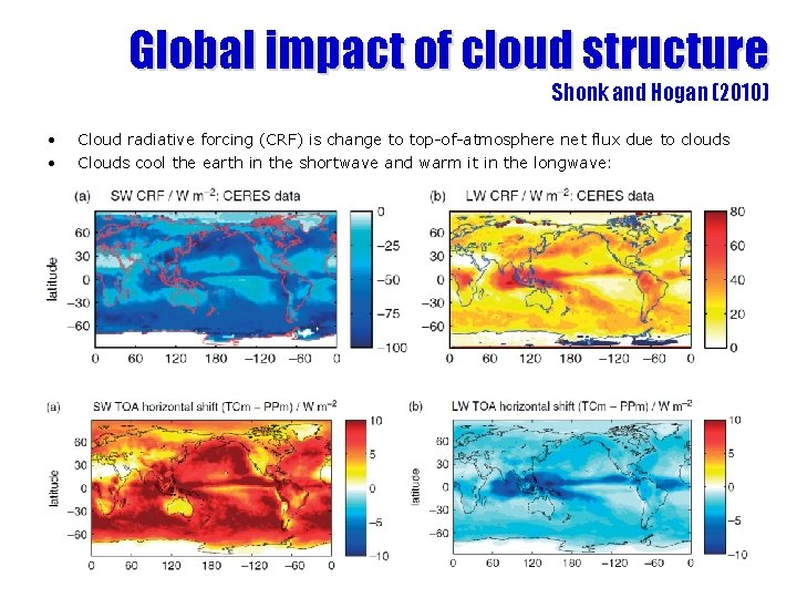
Global impact of cloud structure Shonk and Hogan (2010) • • Cloud radiative forcing (CRF) is change to top-of-atmosphere net flux due to clouds Clouds cool the earth in the shortwave and warm it in the longwave: • Representing horizontal cloud structure reduces absolute CRF by around 12%:

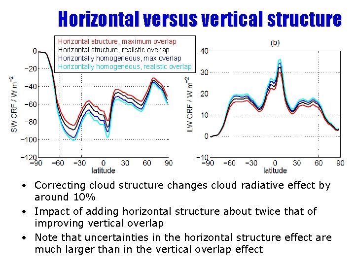
Horizontal versus vertical structure Horizontal structure, maximum overlap Horizontal structure, realistic overlap Horizontally homogeneous, max overlap Horizontally homogeneous, realistic overlap • Correcting cloud structure changes cloud radiative effect by around 10% • Impact of adding horizontal structure about twice that of improving vertical overlap • Note that uncertainties in the horizontal structure effect are much larger than in the vertical overlap effect

Part 5: Remaining challenges • Improve efficiency – Radiation schemes often the slowest part of the model, so may called infrequently and not in every model column • Improve accuracy – Better spectroscopic data, particularly the continuum – Better treatment of upper stratosphere/mesosphere to enable satellite observations here to be assimilated – Evaluate against new observations • Add new processes – – Radiative properties of prognostic aerosols Three dimensional radiative transfer in presence of clouds Non-local-thermodynamic equilibrium for high-top models Cloud inhomogeneity information from cloud scheme

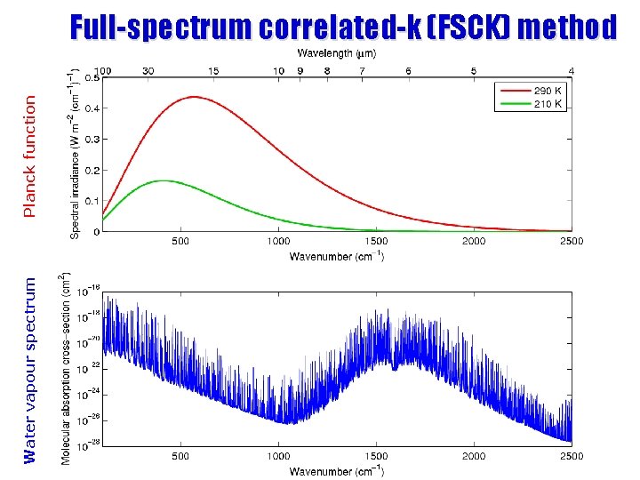
Why do we need bands? 1. Because the Planck function should not vary significantly within a band (Fu & Liou 1992) 2. To minimize number of active gases in each band, due to expense of treating many gases (Mlawer et al. 1997) 3. Because some techniques assume spectral overlap of different gases is random, not valid over large intervals (Edwards 1996) 4. To represent the slow variation of cloud and aerosol absorption and scattering across the spectrum (Ritter & Geleyn 1992) But Modest & Zhang (2002) proposed full-spectrum correlated -k (FSCK) method for combusting gases – – – Their formulation is unnecessarily complex and can be simplified Pawlak et al. (2004) showed that this method works in the shortwave More tricky to apply FSCK to longwave atmospheric radiative transfer, where variations in Planck function and spectral overlap are important

Water vapour spectrum Planck function Full-spectrum correlated-k (FSCK) method

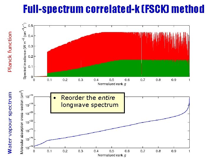
Water vapour spectrum Planck function Full-spectrum correlated-k (FSCK) method • Reorder the entire longwave spectrum

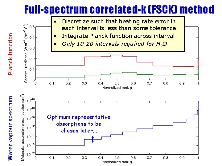
Water vapour spectrum Planck function Full-spectrum correlated-k (FSCK) method • Discretize such that heating rate error in each interval is less than some tolerance • Integrate Planck function across interval • Only 10 -20 intervals required for H 2 O Optimum representative absorptions to be chosen later…

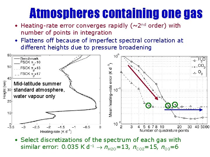
Atmospheres containing one gas • Heating-rate error converges rapidly (~2 nd order) with number of points in integration • Flattens off because of imperfect spectral correlation at different heights due to pressure broadening Mid-latitude summer standard atmosphere, water vapour only • Select discretizations of the spectrum of each gas with similar error: 0. 035 K d-1 n. H 2 O=13, n. CO 2=15, n. O 3=6

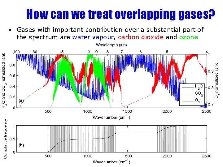
How can we treat overlapping gases? • Gases with important contribution over a substantial part of the spectrum are water vapour, carbon dioxide and ozone

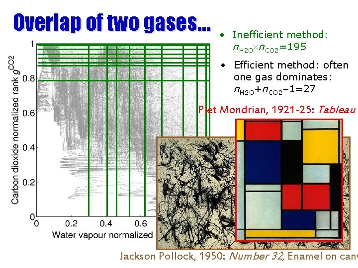
Overlap of two gases… • Inefficient method: n. H 2 O n. CO 2=195 • Efficient method: often one gas dominates: n. H 2 O+n. CO 2– 1=27 Piet Mondrian, 1921 -25: Tableau 2 Jackson Pollock, 1950: Number 32, Enamel on canv

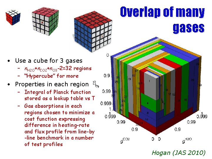
Overlap of many gases • Use a cube for 3 gases – n. H 2 O+n. CO 2+n. O 3 -2=32 regions – “Hypercube” for more • Properties in each region – Integral of Planck function stored as a lookup table vs T – Gas absorptions in each regions chosen to minimize a cost function expressing difference in heating-rate and flux profile from line-by -line benchmark in a number of test profiles Hogan (JAS 2010)

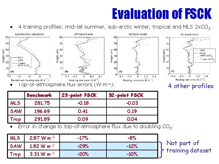
Evaluation of FSCK • 4 training profiles: mid-lat summer, sub-arctic winter, tropical and MLS 2 x. CO 2 • Top-of-atmosphere flux errors (W m-2): Benchmark 23 -point FSCK 4 other profiles 32 -point FSCK MLS 281. 75 – 0. 18 – 0. 03 SAW 196. 69 0. 41 0. 19 Trop 291. 89 0. 04 • Error in change to top-of-atmosphere flux due to doubling CO 2: MLS 2. 87 W m-2 – 17% – 8% SAW 1. 82 W m-2 – 29% – 12% Trop 3. 31 W m-2 – 20% – 10% Not part of training dataset

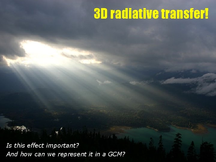
3 D radiative transfer! Is this effect important? And how can we represent it in a GCM?

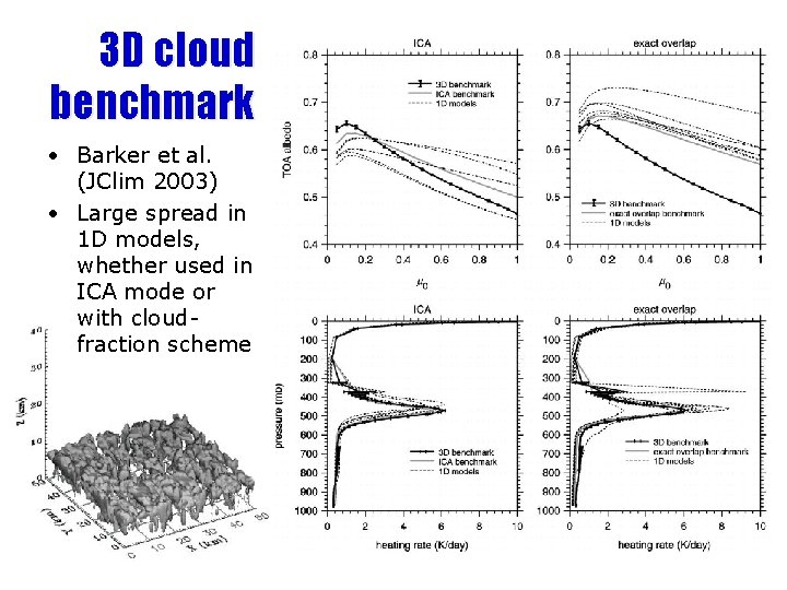
3 D cloud benchmark • Barker et al. (JClim 2003) • Large spread in 1 D models, whether used in ICA mode or with cloudfraction scheme

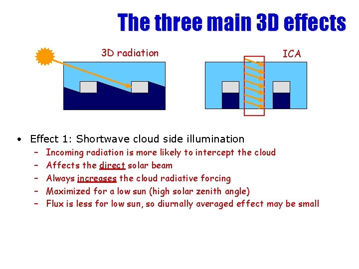
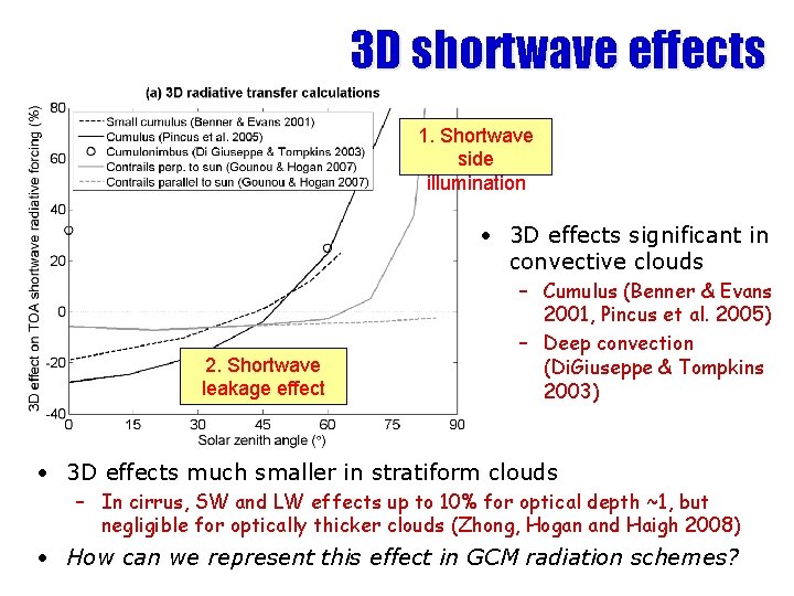
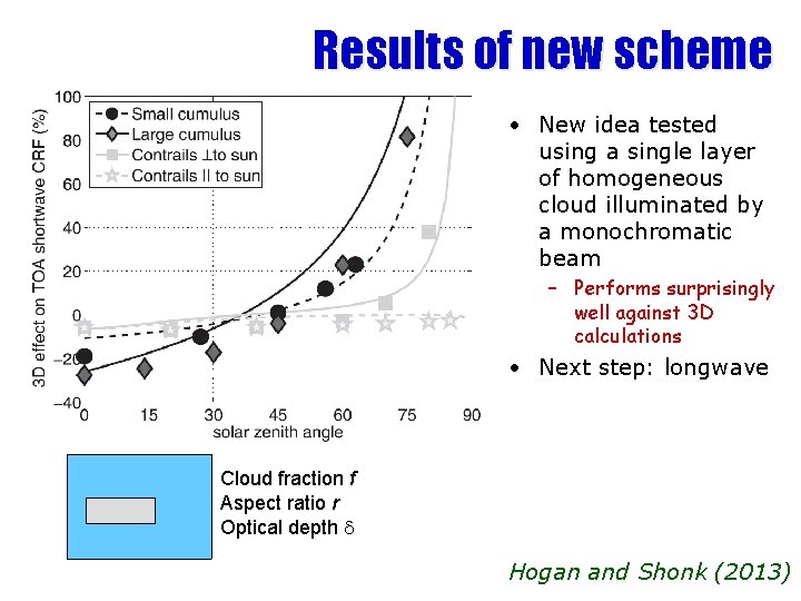
The three main 3 D effects 3 D radiation ICA • Effect 1: Shortwave cloud side illumination – – – Incoming radiation is more likely to intercept the cloud Affects the direct solar beam Always increases the cloud radiative forcing Maximized for a low sun (high solar zenith angle) Flux is less for low sun, so diurnally averaged effect may be small

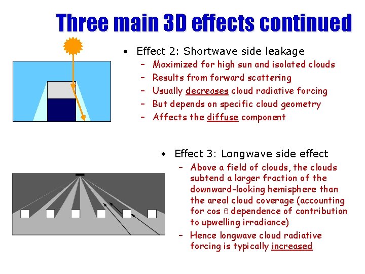
Three main 3 D effects continued • Effect 2: Shortwave side leakage – – – Maximized for high sun and isolated clouds Results from forward scattering Usually decreases cloud radiative forcing But depends on specific cloud geometry Affects the diffuse component • Effect 3: Longwave side effect – Above a field of clouds, the clouds subtend a larger fraction of the downward-looking hemisphere than the areal cloud coverage (accounting for cos q dependence of contribution to upwelling irradiance) – Hence longwave cloud radiative forcing is typically increased

3 D shortwave effects 1. Shortwave side illumination • 3 D effects significant in convective clouds 2. Shortwave leakage effect – Cumulus (Benner & Evans 2001, Pincus et al. 2005) – Deep convection (Di. Giuseppe & Tompkins 2003) • 3 D effects much smaller in stratiform clouds – In cirrus, SW and LW effects up to 10% for optical depth ~1, but negligible for optically thicker clouds (Zhong, Hogan and Haigh 2008) • How can we represent this effect in GCM radiation schemes?

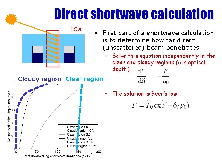
Direct shortwave calculation ICA • First part of a shortwave calculation is to determine how far direct (unscattered) beam penetrates – Solve this equation independently in the clear and cloudy regions (d is optical depth): Cloudy region Clear region – The solution is Beer’s law:

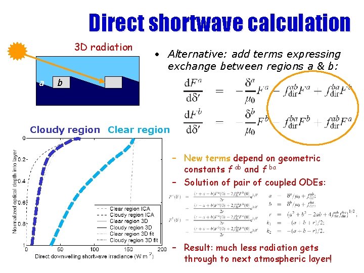
Direct shortwave calculation 3 D radiation a • Alternative: add terms expressing exchange between regions a & b: b Cloudy region Clear region – New terms depend on geometric constants f ab and f ba – Solution of pair of coupled ODEs: – Result: much less radiation gets through to next atmospheric layer!

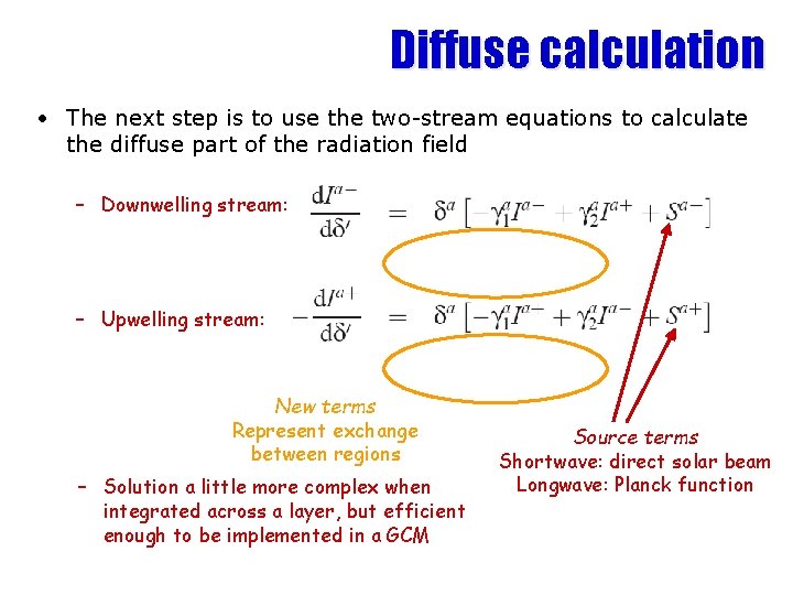
Diffuse calculation • The next step is to use the two-stream equations to calculate the diffuse part of the radiation field – Downwelling stream: – Upwelling stream: New terms Represent exchange between regions – Solution a little more complex when integrated across a layer, but efficient enough to be implemented in a GCM Source terms Shortwave: direct solar beam Longwave: Planck function

Results of new scheme • New idea tested using a single layer of homogeneous cloud illuminated by a monochromatic beam – Performs surprisingly well against 3 D calculations • Next step: longwave Cloud fraction f Aspect ratio r Optical depth d Hogan and Shonk (2013)

Summary • The radiation scheme is a key part of both weather, seasonal and climate forecasts • While the physics is known, there are still challenges in implementing this accurately and efficiently in models • Significant errors still remain, particularly in the representation of clouds