Proteomics Informatics Signal processing I analysis of mass

Proteomics Informatics – Signal processing I: analysis of mass spectra (Week 3)

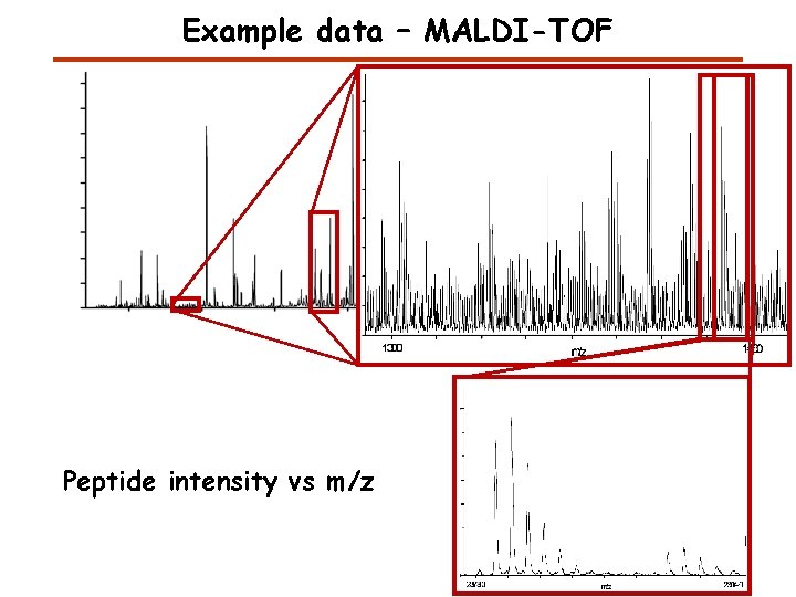
Example data – MALDI-TOF Peptide intensity vs m/z

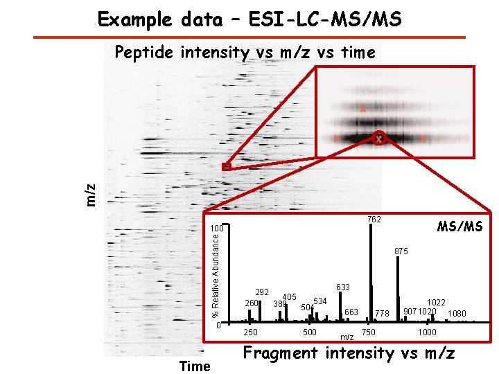
Example data – ESI-LC-MS/MS m/z Peptide intensity vs m/z vs time 762 % Relative Abundance 100 0 Time MS/MS 875 [M+2 H]2+ 292 405 534 260 389 504 250 500 633 663 m/z 778 750 1022 9071020 1080 1000 Fragment intensity vs m/z

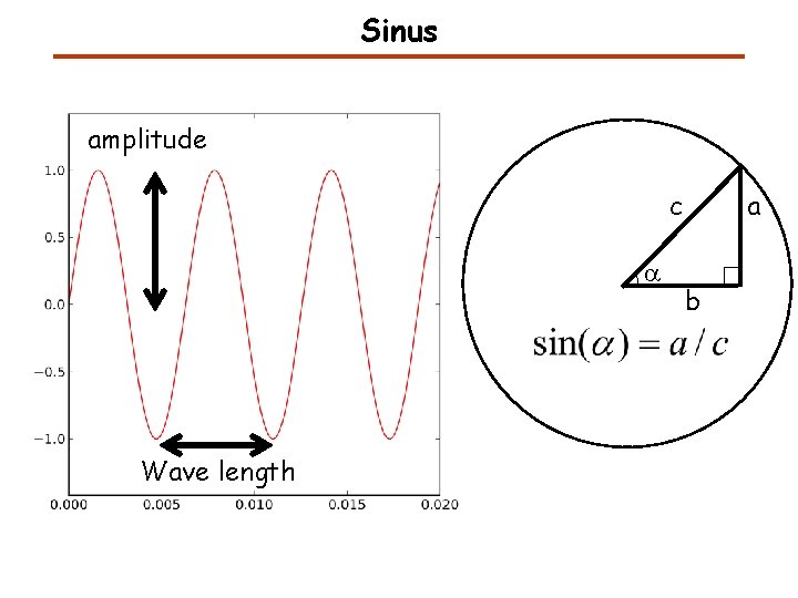
Sinus amplitude c a Wave length a b

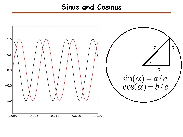
Sinus and Cosinus c a a b

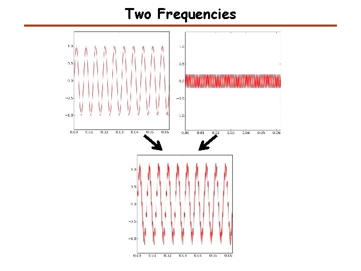
Two Frequencies

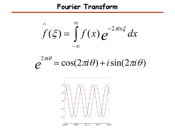
Fourier Transform

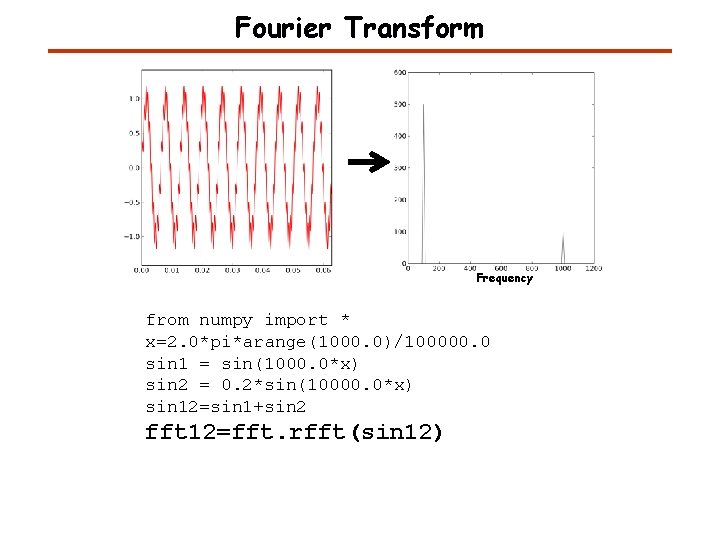
Fourier Transform Frequency from numpy import * x=2. 0*pi*arange(1000. 0)/100000. 0 sin 1 = sin(1000. 0*x) sin 2 = 0. 2*sin(10000. 0*x) sin 12=sin 1+sin 2 fft 12=fft. rfft(sin 12)

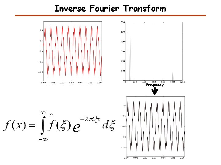
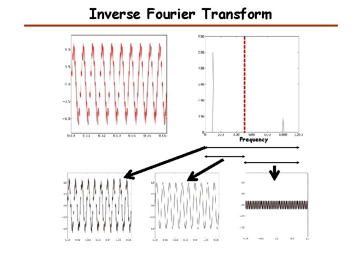
Inverse Fourier Transform Frequency

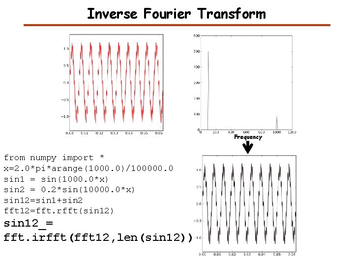
Inverse Fourier Transform Frequency from numpy import * x=2. 0*pi*arange(1000. 0)/100000. 0 sin 1 = sin(1000. 0*x) sin 2 = 0. 2*sin(10000. 0*x) sin 12=sin 1+sin 2 fft 12=fft. rfft(sin 12) sin 12_= fft. irfft(fft 12, len(sin 12))

Inverse Fourier Transform Frequency

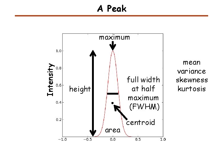
A Peak Intensity maximum full width at half maximum (FWHM) height area centroid mean variance skewness kurtosis

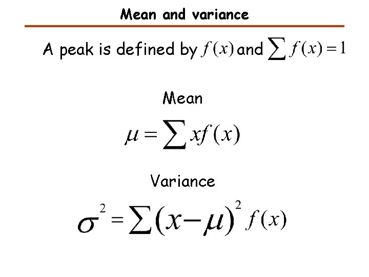
Mean and variance A peak is defined by Mean Variance and

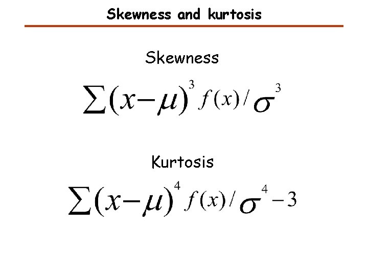
Skewness and kurtosis Skewness Kurtosis

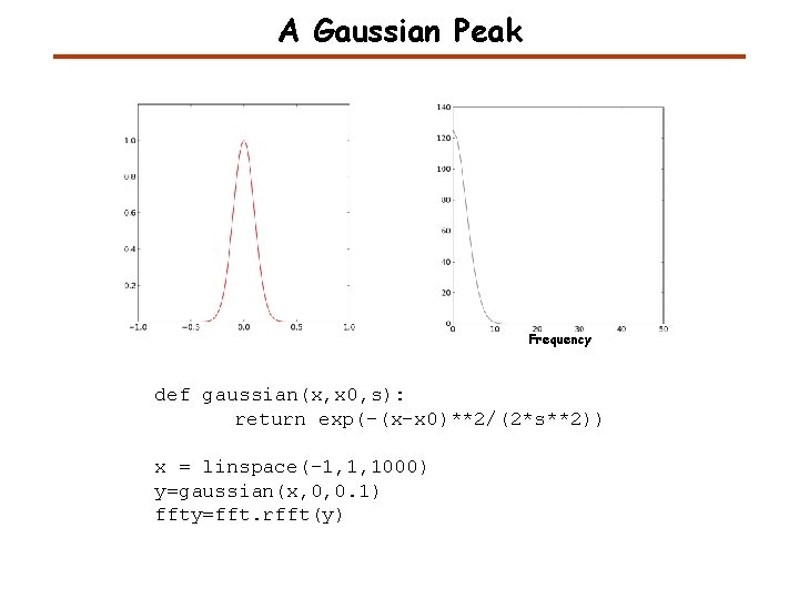
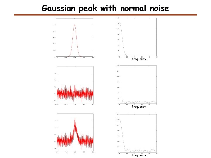
A Gaussian Peak Frequency def gaussian(x, x 0, s): return exp(-(x-x 0)**2/(2*s**2)) x = linspace(-1, 1, 1000) y=gaussian(x, 0, 0. 1) ffty=fft. rfft(y)

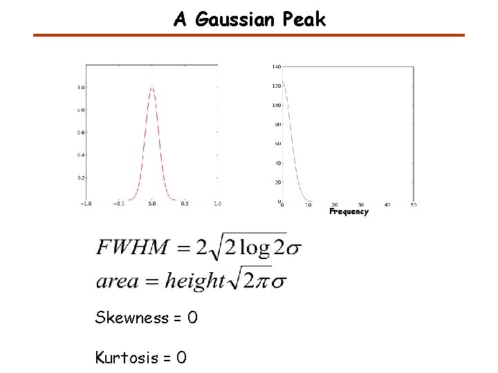
A Gaussian Peak Frequency Skewness = 0 Kurtosis = 0

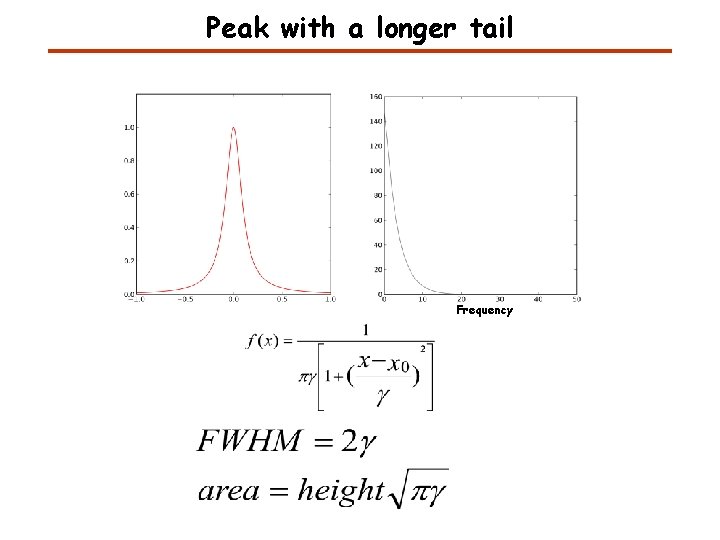
Peak with a longer tail Frequency

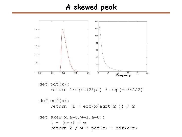
A skewed peak Frequency def pdf(x): return 1/sqrt(2*pi) * exp(-x**2/2) def cdf(x): return (1 + erf(x/sqrt(2))) / 2 def skew(x, e=0, w=1, a=0): t = (x-e) / w return 2 / w * pdf(t) * cdf(a*t)

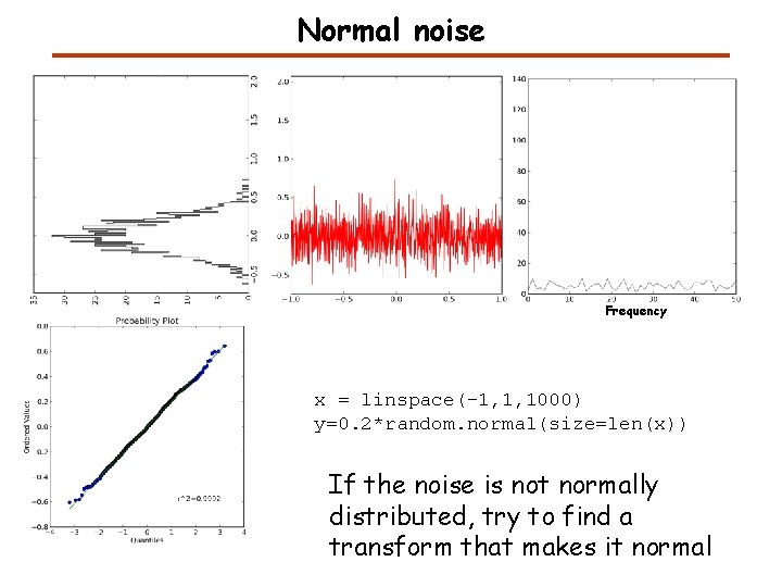
Normal noise Frequency x = linspace(-1, 1, 1000) y=0. 2*random. normal(size=len(x)) If the noise is not normally distributed, try to find a transform that makes it normal

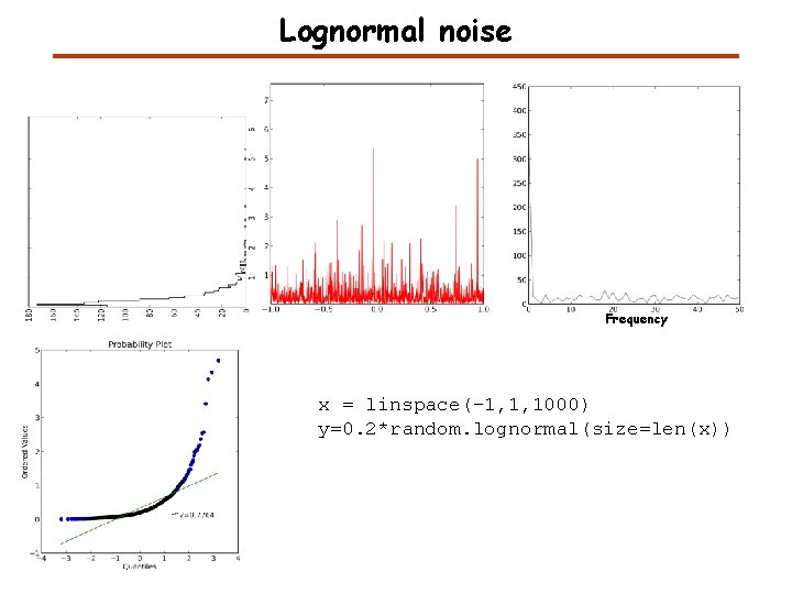
Lognormal noise Frequency x = linspace(-1, 1, 1000) y=0. 2*random. lognormal(size=len(x))

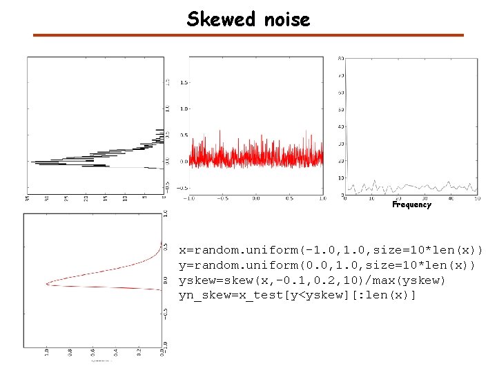
Skewed noise Frequency x=random. uniform(-1. 0, size=10*len(x)) y=random. uniform(0. 0, 1. 0, size=10*len(x)) yskew=skew(x, -0. 1, 0. 2, 10)/max(yskew) yn_skew=x_test[y<yskew][: len(x)]

Gaussian peak with normal noise Frequency

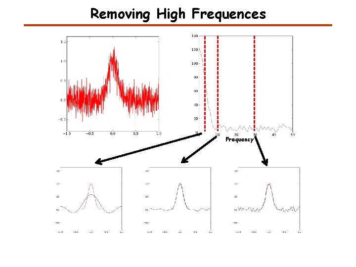
Removing High Frequences Frequency

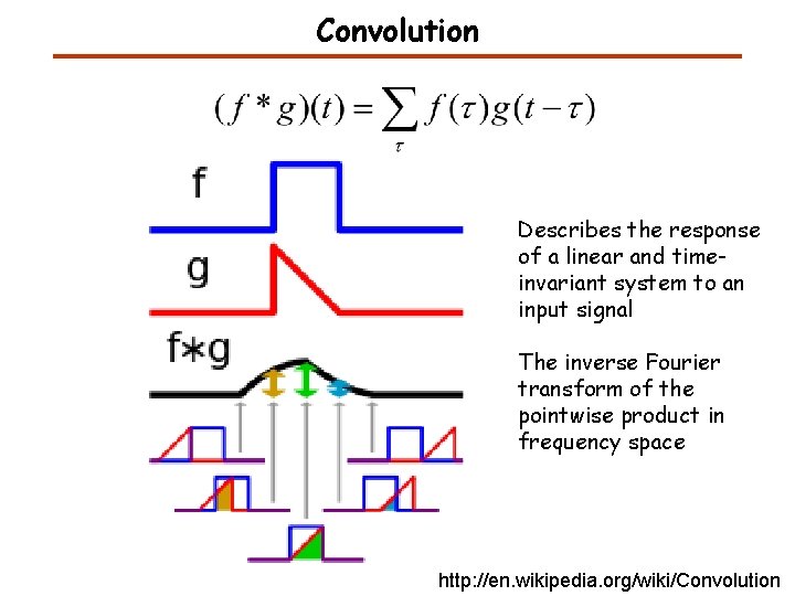
Convolution Describes the response of a linear and timeinvariant system to an input signal The inverse Fourier transform of the pointwise product in frequency space http: //en. wikipedia. org/wiki/Convolution

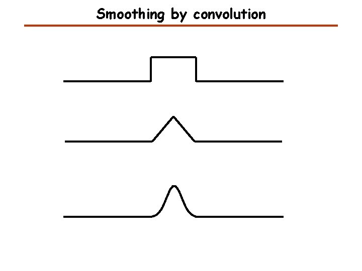
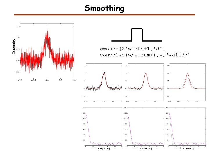
Smoothing by convolution

Intensity Smoothing w=ones(2*width+1, 'd') convolve(w/w. sum(), y, 'valid‘) Frequency

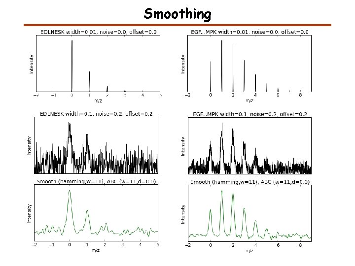
Smoothing

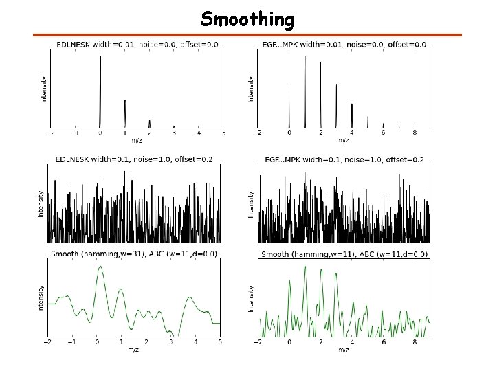
Smoothing

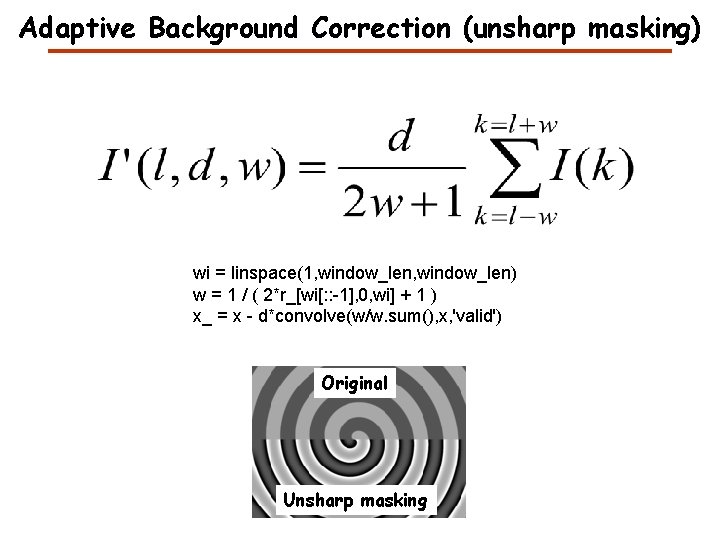
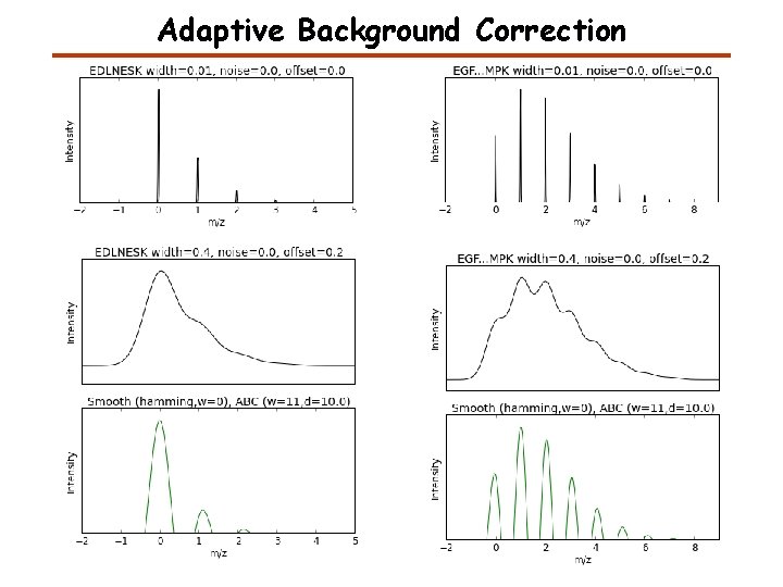
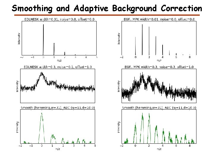
Adaptive Background Correction (unsharp masking) wi = linspace(1, window_len) w = 1 / ( 2*r_[wi[: : -1], 0, wi] + 1 ) x_ = x - d*convolve(w/w. sum(), x, 'valid') Original Unsharp masking

Adaptive Background Correction

Smoothing and Adaptive Background Correction

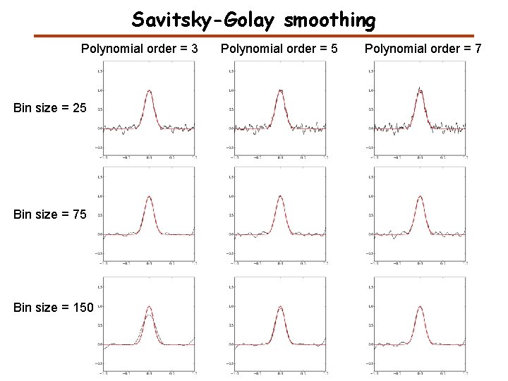
Savitsky-Golay smoothing Polynomial order = 3 Bin size = 25 Bin size = 75 Bin size = 150 Polynomial order = 5 Polynomial order = 7

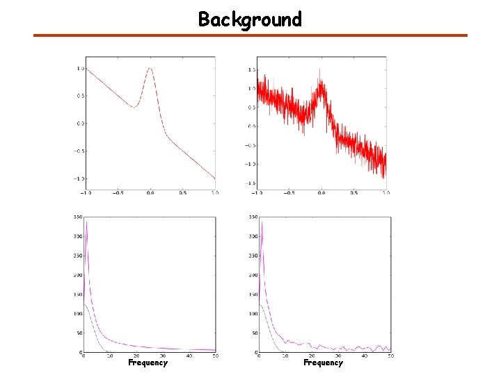
Background Frequency

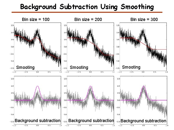
Background Subtraction Using Smoothing Bin size = 100 Smooting Background subtraction Bin size = 200 Smooting Background subtraction Bin size = 300 Smooting Background subtraction

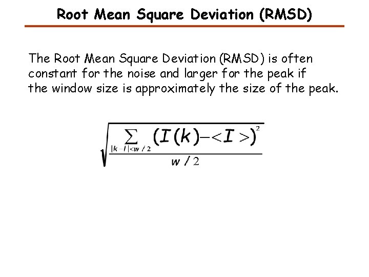
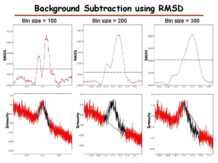
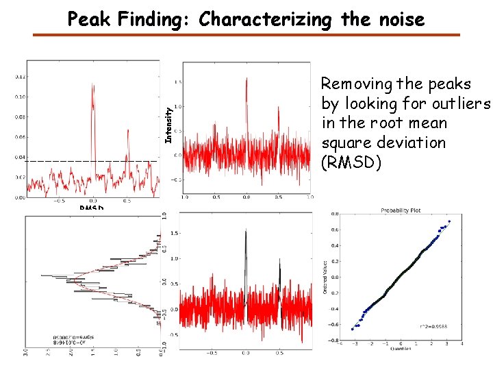
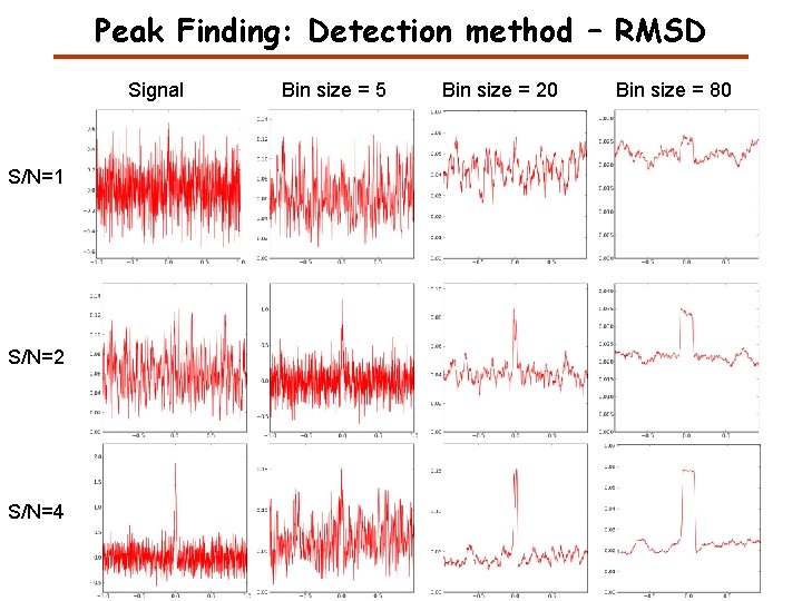
Root Mean Square Deviation (RMSD) The Root Mean Square Deviation (RMSD) is often constant for the noise and larger for the peak if the window size is approximately the size of the peak.

Background Subtraction using RMSD Bin size = 300 Intensity RMSD Bin size = 200 Intensity RMSD Bin size = 100

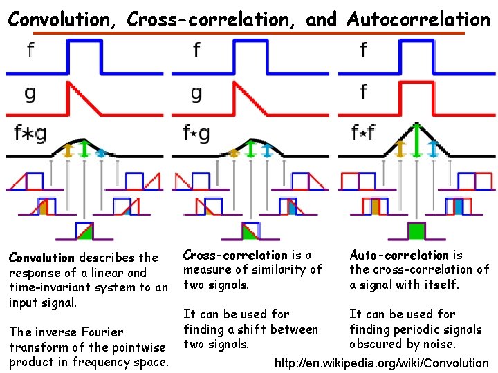
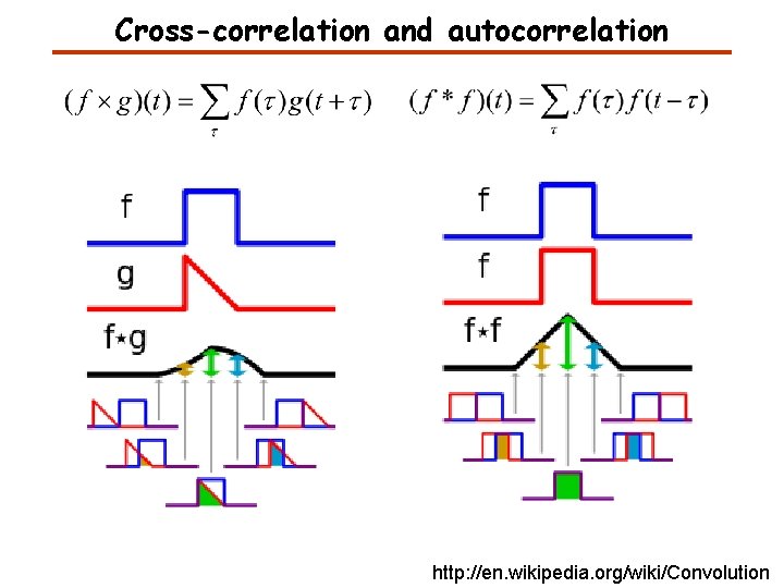
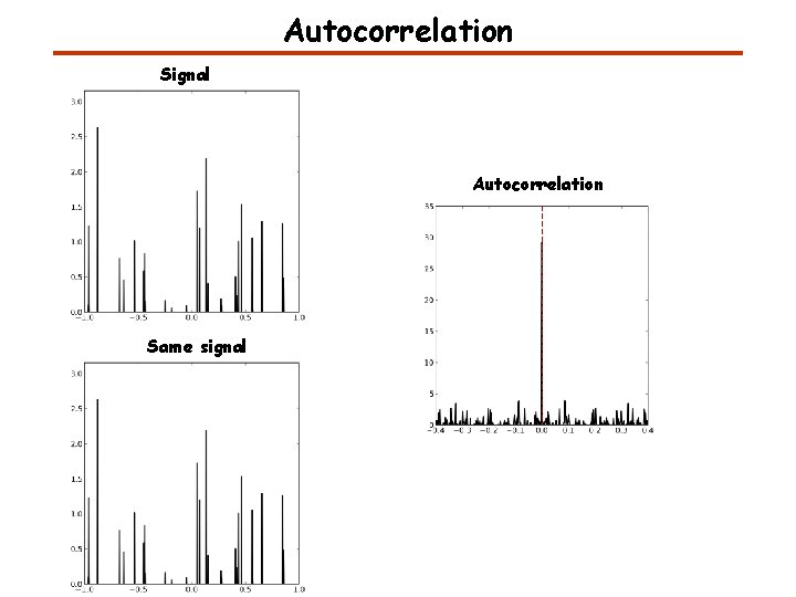
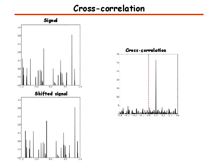
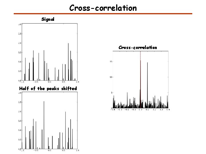
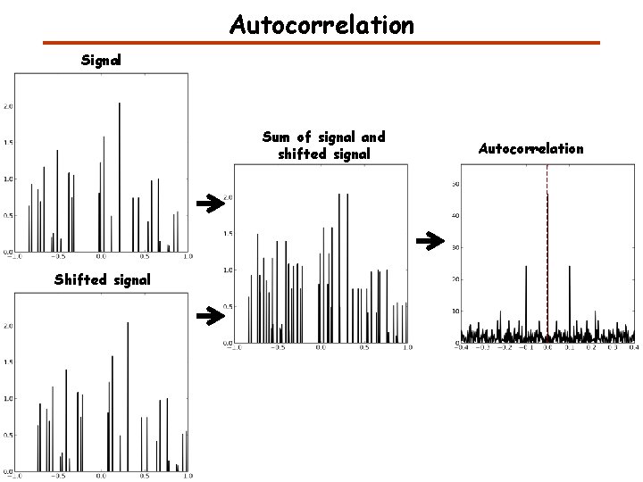
Convolution, Cross-correlation, and Autocorrelation Convolution describes the response of a linear and time-invariant system to an input signal. The inverse Fourier transform of the pointwise product in frequency space. Cross-correlation is a measure of similarity of two signals. Auto-correlation is the cross-correlation of a signal with itself. It can be used for finding a shift between two signals. It can be used for finding periodic signals obscured by noise. http: //en. wikipedia. org/wiki/Convolution

Cross-correlation and autocorrelation http: //en. wikipedia. org/wiki/Convolution

Autocorrelation Signal Autocorrelation Same signal

Cross-correlation Signal Cross-correlation Shifted signal

Cross-correlation Signal Cross-correlation Half of the peaks shifted

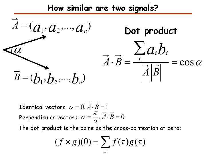
How similar are two signals? Dot product Identical vectors: Perpendicular vectors: The dot product is the came as the cross-correation at zero:

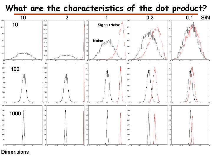
What are the characteristics of the dot product? 10 10 3 1 Signal+Noise 100 1000 Dimensions 0. 3 0. 1 S/N

Autocorrelation Signal Sum of signal and shifted signal Shifted signal Autocorrelation

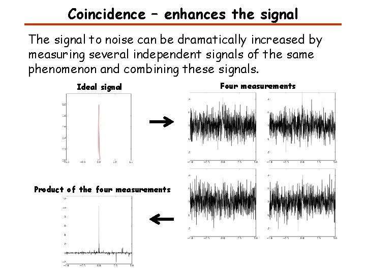
Coincidence – enhances the signal The signal to noise can be dramatically increased by measuring several independent signals of the same phenomenon and combining these signals. Ideal signal Product of the four measurements Four measurements

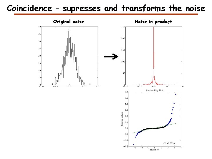
Coincidence – supresses and transforms the noise Original noise Noise in product

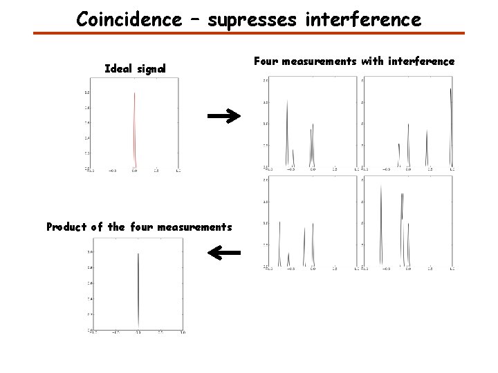
Coincidence – supresses interference Ideal signal Product of the four measurements Four measurements with interference

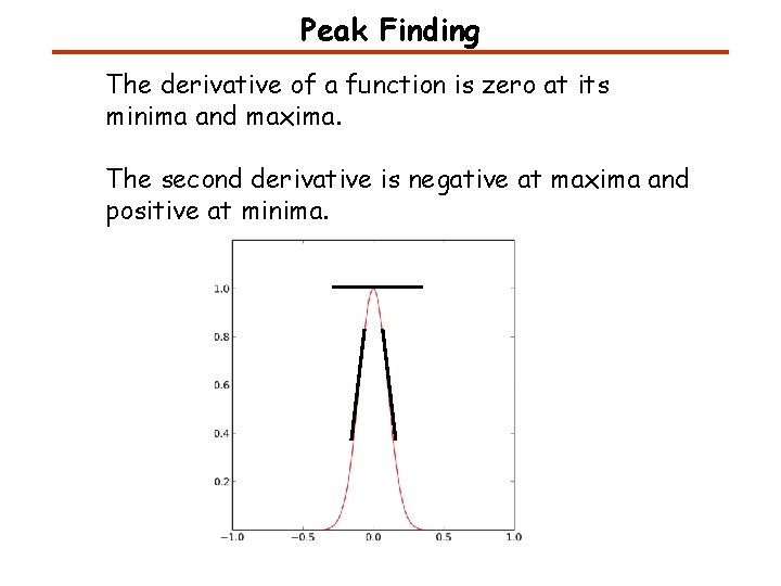
Peak Finding The derivative of a function is zero at its minima and maxima. The second derivative is negative at maxima and positive at minima.

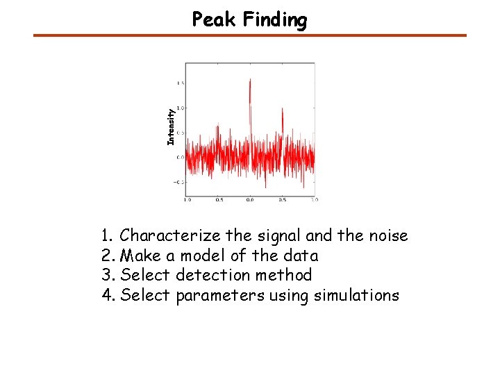
Intensity Peak Finding 1. Characterize the signal and the noise 2. Make a model of the data 3. Select detection method 4. Select parameters using simulations

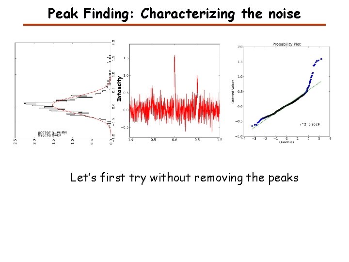
Intensity Peak Finding: Characterizing the noise Let’s first try without removing the peaks

Intensity Peak Finding: Characterizing the noise RMSD Removing the peaks by looking for outliers in the root mean square deviation (RMSD)

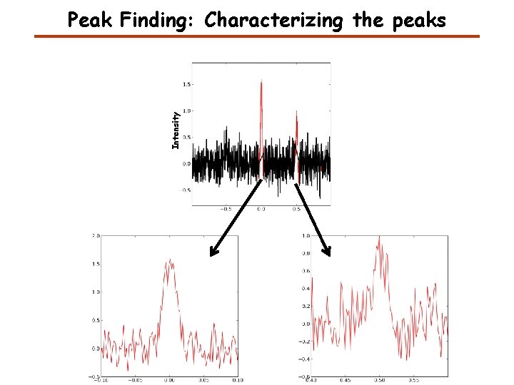
Intensity Peak Finding: Characterizing the peaks

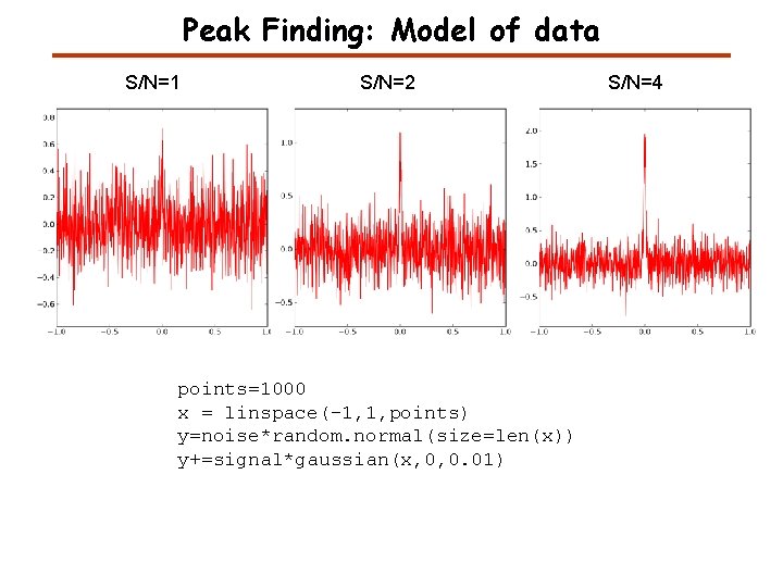
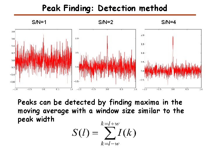
Peak Finding: Model of data S/N=1 S/N=2 points=1000 x = linspace(-1, 1, points) y=noise*random. normal(size=len(x)) y+=signal*gaussian(x, 0, 0. 01) S/N=4

Peak Finding: Detection method S/N=1 S/N=2 S/N=4 Peaks can be detected by finding maxima in the moving average with a window size similar to the peak width

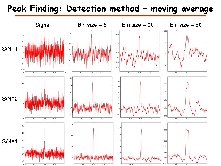
Peak Finding: Detection method – moving average Signal S/N=1 S/N=2 S/N=4 Bin size = 5 Bin size = 20 Bin size = 80

Peak Finding: Detection method – RMSD Signal S/N=1 S/N=2 S/N=4 Bin size = 5 Bin size = 20 Bin size = 80

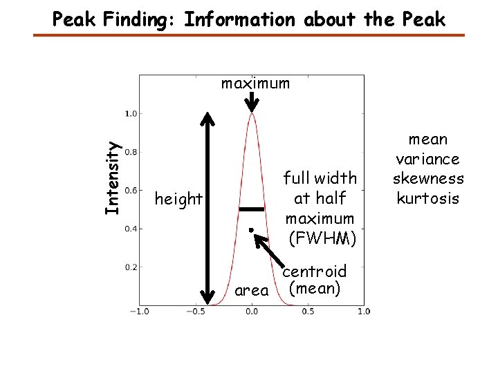
Peak Finding: Information about the Peak Intensity maximum height full width at half maximum (FWHM) centroid area (mean) mean variance skewness kurtosis

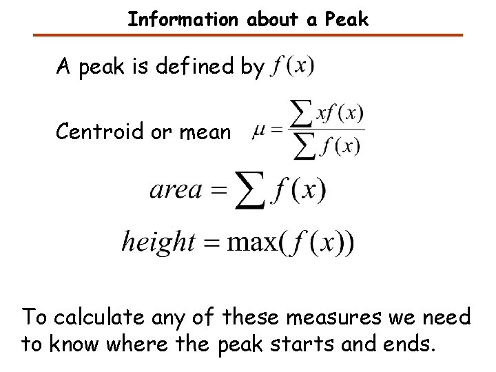
Information about a Peak A peak is defined by Centroid or mean To calculate any of these measures we need to know where the peak starts and ends.

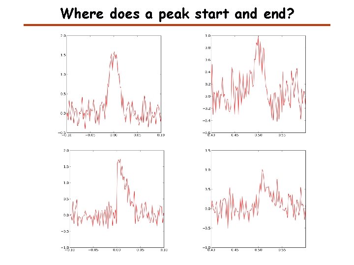
Where does a peak start and end?

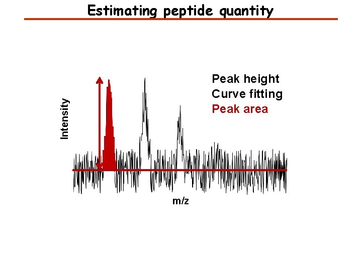
Estimating peptide quantity Intensity Peak height Curve fitting Peak area m/z

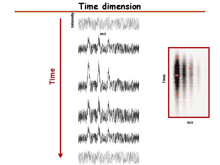
Intensity Time dimension Time m/z

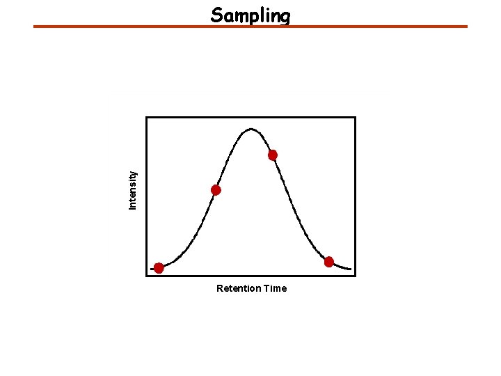
Intensity Sampling Retention Time

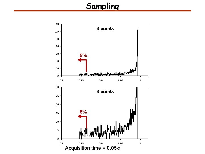
Sampling 5% 5% Acquisition time = 0. 05 s

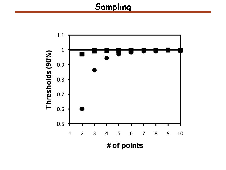
Sampling

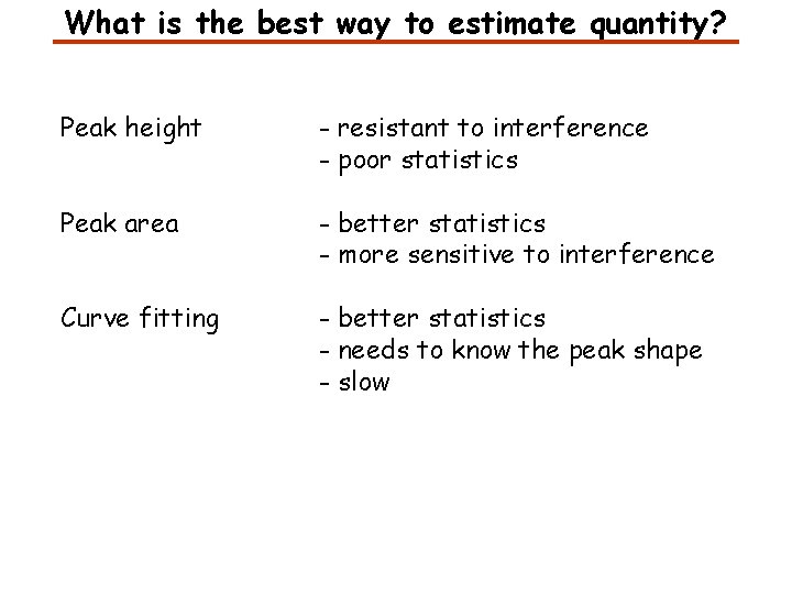
What is the best way to estimate quantity? Peak height - resistant to interference - poor statistics Peak area - better statistics - more sensitive to interference Curve fitting - better statistics - needs to know the peak shape - slow

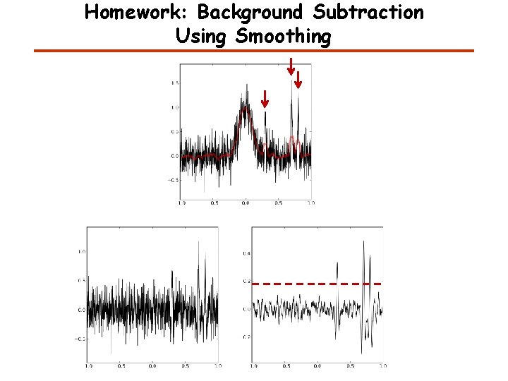
Homework: Background Subtraction Using Smoothing

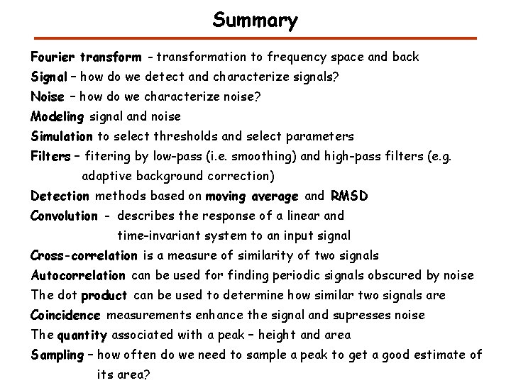
Summary Fourier transform - transformation to frequency space and back Signal – how do we detect and characterize signals? Noise – how do we characterize noise? Modeling signal and noise Simulation to select thresholds and select parameters Filters – fitering by low-pass (i. e. smoothing) and high-pass filters (e. g. adaptive background correction) Detection methods based on moving average and RMSD Convolution - describes the response of a linear and time-invariant system to an input signal Cross-correlation is a measure of similarity of two signals Autocorrelation can be used for finding periodic signals obscured by noise The dot product can be used to determine how similar two signals are Coincidence measurements enhance the signal and supresses noise The quantity associated with a peak – height and area Sampling – how often do we need to sample a peak to get a good estimate of its area?

Proteomics Informatics – Signal processing I: analysis of mass spectra (Week 3)