Proteiinianalyysi 5 Rakenteiden vertailu ja luokittelu http www


 – Comparing conformations • Angles,")


 B A")
: Distance Between an Atom in 2 Structures")
: RMS Distance Between Aligned Atoms in 2 Structures")
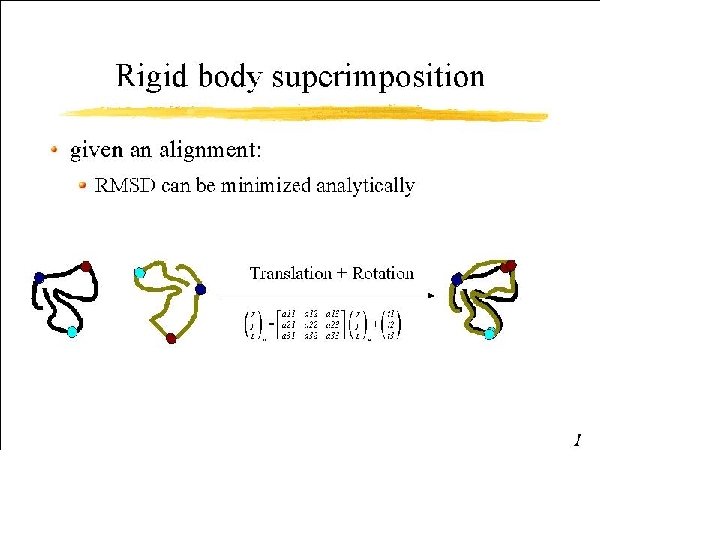
: Rigid-Body Rotation and Translation of One Structure (B)")
 Make a Similarity Matrix (Like Dot Plot)")
 Make a Similarity Matrix (Generalized Similarity Matrix) i • PAM(A,")
 Similarity Matrix for Structural Alignment • Structural Alignment – Similarity")
: Dynamic Programming, Start Computing the Sum Matrix new_value_cell(R, C) <= cell(R, C)")
: Dynamic Programming, Keep Going")
: Dynamic Programming, Sum Matrix All Done")
: Traceback Find Best Score (8) and Trace Back A B C N")
 • Use Alignment to LSQ Fit")

, Iterate Until Convergence 1 Compute Sim. Matrix 2 Align via Dyn.")


![P-values 1 2 [ e. g. P(score s>392) = 1% chance] 3 • Significance](https://slidetodoc.com/presentation_image_h2/b7d56af6e03cf7d185bf383bab33178f/image-50.jpg "P-values 1 2 [ e. g. P(score s>392) = 1% chance] 3 • Significance")


")


 All")


 1. Globin-like (2) core: 6")

 (117) Mainly parallel")
-binding Rossmann-fold domains (1) core: 3 layers,")


, T-level • Structures are grouped into fold families at this level")


 5 -stranded propeller")
 Irregular")
 jätetty")


- Slides: 111
Proteiinianalyysi 5 Rakenteiden vertailu ja luokittelu http: //www. bioinfo. biocenter. helsinki. fi/downlo ads/teaching/spring 2006/proteiinianalyysi
Why compare 3 D structures? • Structure is more conserved than sequence • Structure comparison can reveal evolutionary relationships not easily detected by sequence comparison – Aspects of function are inherited down evolutionary lineages
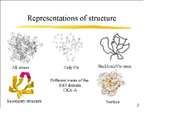
How to compare 3 D structures • • Representation of structure Useful measure of structural similarity Optimization algorithm Assessment of significance
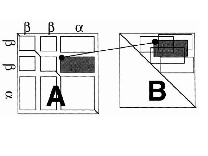
Representation of protein structure • Protein structures have to be represented in some coordinate independent space to make them comparable. One possible representation is the so-called distance matrix, which is a two-dimensional matrix containing all pairwise distance between all Cα atoms of the protein backbone. This can also be represented as a set of overlapping sub-matrices spanning only fragments of the protein. Another possible representation is the reduction of the protein structure to the level of secondary structure elements (SSEs), which can be represented as vectors, and can carry additional information about relationships to other SSEs, as well as about certain biophysical properties.
Depicting Protein Structure: Sperm Whale Myoglobin
Topology diagrams • There a number of ways to represent the folding of a protein and the arrangement of secondary structure elements within the tertiary structure. While these simplifications don't show the sidechain and mainchain interactions that hold the structures together, they do reveal the folding pattern. Examination of such diagrams reveals recurring structural patterns in protein folding.
Molecular Biology Information: Protein Structure Details • Statistics on Number of XYZ triplets – 200 residues/domain -> 200 CA atoms, separated by 3. 8 A – Avg. Residue is Leu: 4 backbone atoms + 4 sidechain atoms, 150 cubic A • => ~1500 xyz triplets (=8 x 200) per protein domain ATOM ATOM ATOM 1 2 3 4 5 6 7 8 9 10 11 12 C O CH 3 N CA C O CB OG N CA C ACE ACE SER SER SER ARG ARG 0 0 0 1 1 1 2 2 2 9. 401 10. 432 8. 876 8. 753 9. 242 10. 453 10. 593 8. 052 7. 294 11. 360 12. 548 13. 502 30. 166 30. 832 29. 767 29. 755 30. 200 29. 500 29. 607 30. 189 31. 409 28. 819 28. 316 29. 501 60. 595 60. 722 59. 226 61. 685 62. 974 63. 579 64. 814 63. 974 63. 930 62. 827 63. 532 63. 500 1. 00 1. 00 49. 88 50. 35 50. 04 49. 13 46. 62 41. 99 43. 24 53. 00 57. 79 36. 48 30. 20 25. 54 1 GKY 1 GKY 1 GKY 67 68 69 70 71 72 73 74 75 76 77 78 1444 1445 1446 1447 1448 1449 1450 CB CG CD CE NZ OXT LYS LYS 186 186 13. 836 12. 422 11. 531 11. 452 10. 735 16. 887 22. 263 22. 452 21. 198 20. 402 21. 104 23. 841 57. 567 58. 180 58. 185 56. 860 55. 811 56. 647 1. 00 55. 06 53. 45 49. 88 48. 15 48. 41 62. 94 1 GKY 1510 1 GKY 1511 1 GKY 1512 1 GKY 1513 1 GKY 1514 1 GKY 1515 1 GKY 1516 . . . ATOM ATOM TER
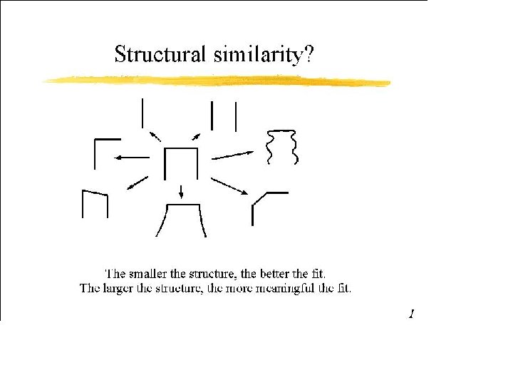
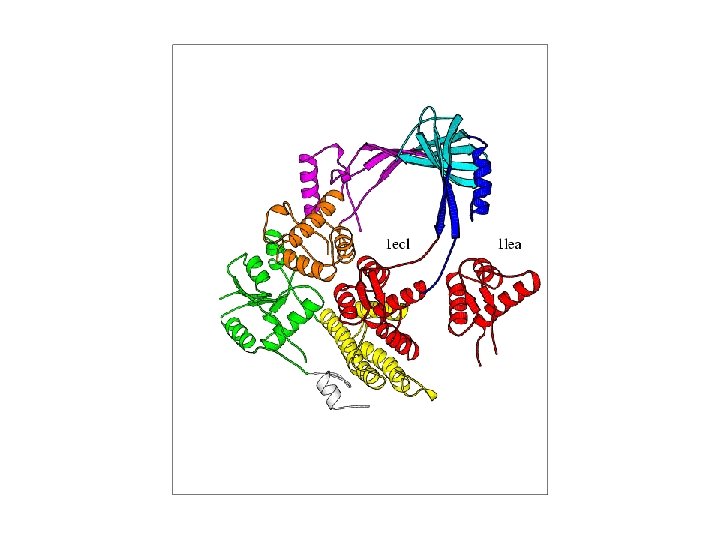
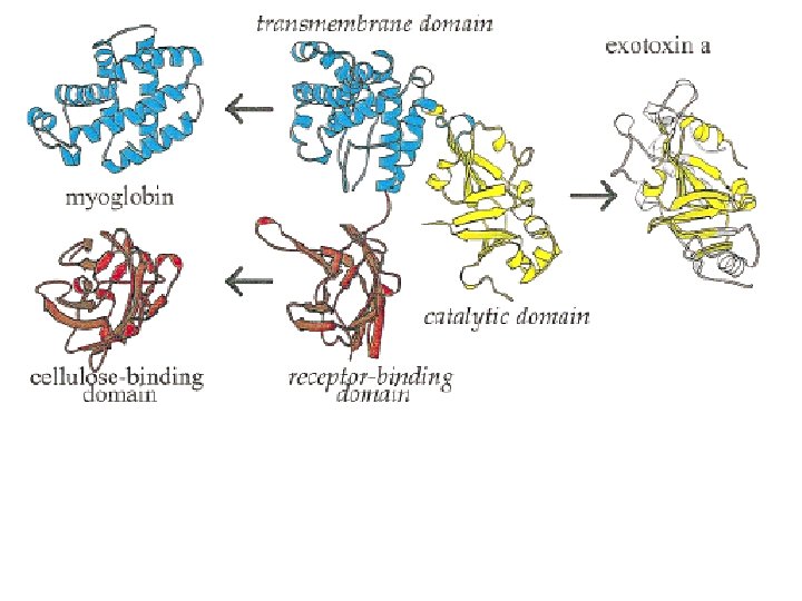
Some Similarities are Readily Apparent others are more Subtle Easy: Globins 125 res. , ~1. 5 Å Tricky: Very Subtle: G 3 P-dehydro. Ig C & V genase, C-term. Domain >5 Å 85 res. , ~3 Å
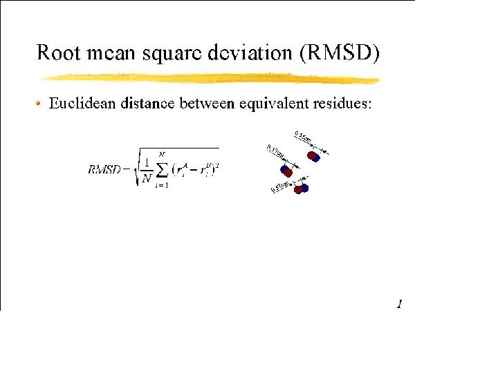
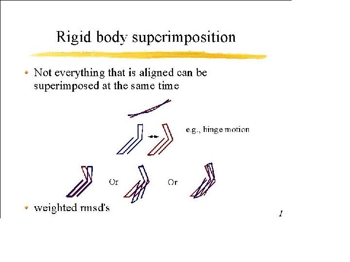
Measures of protein structure similarity • Root-mean-square deviation (RMSD) – Comparing conformations • Angles, distances between SSEs – Graph isomorphism • Similarity scores based on inter-molecular distances (dynamic programming) – Soap-film distance metric • Weighted sum of intra-molecular distances – Dali (distance matrix alignment)
RMSD: positional deviations
Soap film metric = surface area between two C-alpha traces
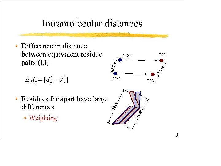
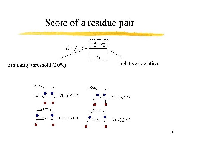
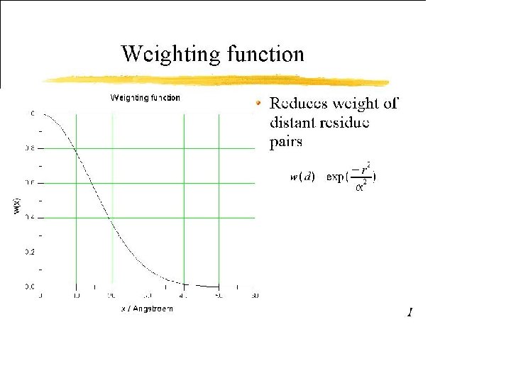
Distance difference matrix Relative distance difference, compared to a threshold of similarity, weighted by an envelope function
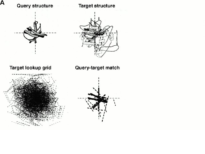
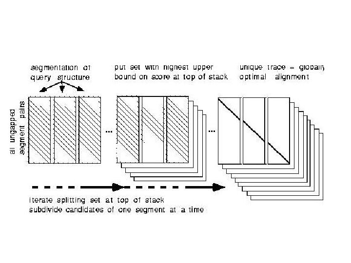
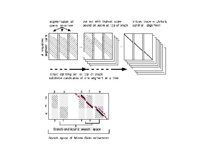
Shift 0 Shift 5 Shift 0 & Shift 5 Extending distance matrix alignment
Comparison and Optimization • In the case of distance matrix representation, the comparison algorithm breaks down the distance matrices into regions of overlap, which are then again combined if there is overlap between adjacent fragments, thereby extending the alignment. If the SSE representation is chosen, there are several possibilities. One can search for the maximum ensemble of equivalent SSE pairs using algorithms to solve the maximum clique problem from graph theory. Other approaches employ dynamic programming or combinatorial simulated annealing.
Maximizing the number of residues that fit within an RMSD limit • Iterative procedure – Initial alignment superimposition – Inter-molecular distance measure – Use dynamic programming to refine alignment • Kolodny & Linial – Gives solution within bound – Too computationally heavy for routine use
Fitting largest number of residues under an RMSD cutoff • Recently an approximate polynomial time algorithm for protein structural alignment was presented by Kolodny & Linial. This is in contrast to a rumour saying that the structural alignment problem is NP-hard. Although polynomial, it is still a very expensive algorithm (O(n 10 / ε 6)). Thus, all current programs employ heuristic methods. Different programs do not necessarily produce exactly the same results for the same alignment problem.
RMS Superposition (1) B A
RMS Superposition (2): Distance Between an Atom in 2 Structures
RMS Superposition (3): RMS Distance Between Aligned Atoms in 2 Structures
RMS Superposition (4): Rigid-Body Rotation and Translation of One Structure (B)
Alignment (1) Make a Similarity Matrix (Like Dot Plot)
Structural Alignment (1 b) Make a Similarity Matrix (Generalized Similarity Matrix) i • PAM(A, V) = 0. 5 – Applies at every position • S(aa @ i, aa @ J) – Specific Matrix for each pair of residues i in protein 1 and J in protein 2 – Example is Y near N-term. matches any C-term. residue (Y at J=2) • S(i, J) – Doesn’t need to depend on a. a. identities at all! – Just need to make up a score for matching residue i in protein 1 with residue J in protein 2 J
Structural Alignment (1 c*) Similarity Matrix for Structural Alignment • Structural Alignment – Similarity Matrix S(i, J) depends on the 3 D coordinates of residues i and J – Distance between CA of i and J – M(i, j) = 100 / (5 + d 2) • Threading – S(i, J) depends on the how well the amino acid at position i in protein 1 fits into the 3 D structural environment at position J of protein 2
Alignment (2): Dynamic Programming, Start Computing the Sum Matrix new_value_cell(R, C) <= cell(R, C) { + Max[ cell (R+1, C+1), { cells(R+1, C+2 to C_max), { cells(R+2 to R_max, C+2) { ] Old value, either 1 or 0 } Diagonally Down, no gaps } Down a row, making col. gap } Down a col. , making row gap }
Alignment (3): Dynamic Programming, Keep Going
Alignment (4): Dynamic Programming, Sum Matrix All Done
Alignment (5): Traceback Find Best Score (8) and Trace Back A B C N Y - R Q C L C R - P M A Y C - Y N R - C K C R B P
In Structural Alignment, Not Yet Done (Step 6*) • Use Alignment to LSQ Fit Structure B onto Structure A – However, movement of B will now change the Similarity Matrix • This Violates Fundamental Premise of Dynamic Programming – Way Residue at i is aligned can now affect previously optimal alignment of residues (from 1 to i-1) ACSQRP--LRV-SH -R SENCV A-SNKPQLVKLMTH VK DFCV-
How central idea of dynamic programming is violated in structural alignment
Structural Alignment (7*), Iterate Until Convergence 1 Compute Sim. Matrix 2 Align via Dyn. Prog. 3 RMS Fit Based on Alignment 4 Move Structure B 5 Re-compute Sim. Matrix 6 If changed from #1, GOTO #2
Soap film metric = surface area between two C-alpha traces The same iterative procedure can be used with soap film metric
SSAP, Double dynamic programming • Program used for CATH database • Lower level – Fix coordinate frame on the backbone of one residue – Align residue environments • Upper level – Cumulates scores of similarities in residue environments
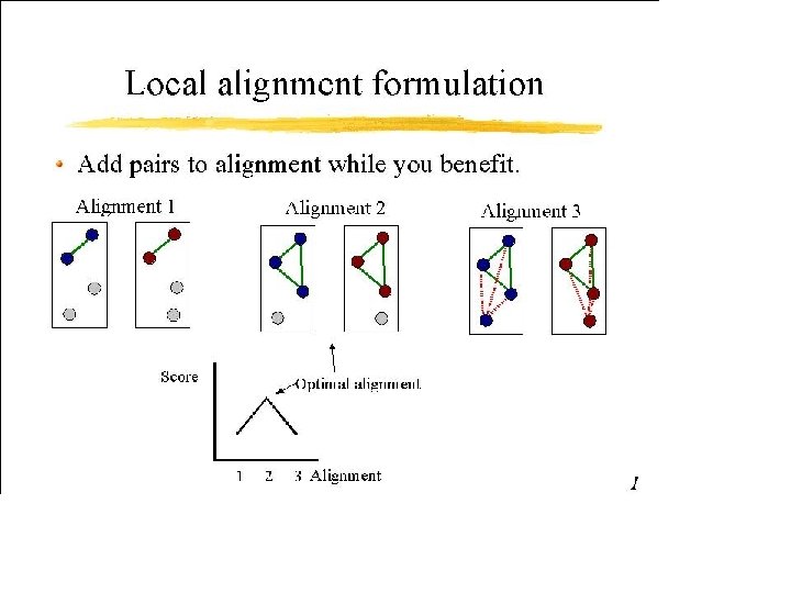
Distance matrix alignment problem • Find a set of one-to-one correspondences of residues (or C-alpha atoms or C-beta atoms or secondary structure vectors or …) that maximize your chosen similarity measure – Sequential alignment • Exact solutions are computationally hard – Sum of pairs score – Heuristics speed up the search – Approximate measures
Probability of SSE matching • VAST – Extreme value distribution a la Blast – Probability of superimposing N secondary structure elements by picking elements randomly ~10 -8 – Alternative element pair combinations ~104 – Likelihood of alignment is the product ~ 10 -8 x 104 = 10 -4
Score S at End Just Like SW Score, but also have final RMS S = Total Score S(i, j) = similarity matrix score for aligning i and j Sum is carried out over all aligned i and j n = number of gaps (assuming no gap ext. penalty) G = gap penalty
P-values 1 2 [ e. g. P(score s>392) = 1% chance] 3 • Significance Statistics – For sequences, originally used in Blast (Karlin-Altschul). Then in FASTA, &c. – Extrapolated Percentile Rank: How does a Score Rank Relative to all Other Scores? • Our Strategy: Fit to Observed Distribution 1)All-vs-All comparison 2)Graph Distribution of Scores in 2 D (N dependence); 1 K x 1 K families -> ~1 M scores; ~2 K included TPs 3)Fit a function r(S) to TN distribution (TNs from scop); Integrating r gives P(s>S), the CDF, chance of getting a score better than threshold S randomly 4) Use same formalism for sequence & structure
Scores from Structural Alignment Distributed Just Like Ones from Sequence Alignment (E. V. D. )
Dali Z-score
Meaning of Dali Z-score
Protein domains/modules • globular • independently foldable • occur in different contexts
Domains via the contact matrix
Protein Unfolding Units • Contact matrix • Binary decomposition
Dali domains
Structure classification • Organise structures in PDB hierarchically • SCOP (Alexey Murzin, LMB Cambridge) – Manually checked – “Dali is useful” • CATH (Christine Orengo, UCL London) – Semi-automatic – Based on SSAP • Dali DB (Helsinki) – Automatic – All-against-all comparison using Dali
Domains • SCOP: manual – no cut if unique combination • CATH: based on three independent algorithms for domain recognition (DETECTIVE (Swindells, 1995), PUU (Holm & Sander, 1994) and DOMAK (Siddiqui and Barton, 1995). This currently allows approximately 53% of the proteins (i. e. those for which these algorithms agree) to be defined as single or multidomain proteins automatically. The remaining structures are assigned domain definitions manually, by choosing what was determined to be the best assignment made by one of the algorithms, a new assignment, or an alternative assignment obtained from the literature. • Dali: recurrence optimization
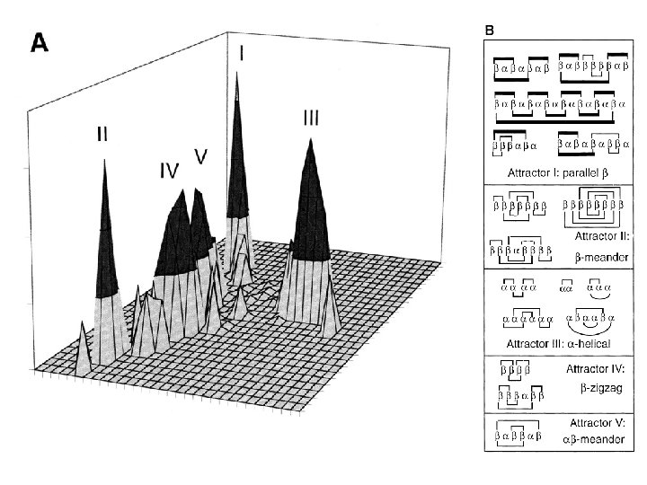
Dali classification • All-against-all structure comparison • • Class – by proximity to archetypes Fold – by cutting fold dendrogram at Z=2 Superfamily – by clustering Family – by sequence identity
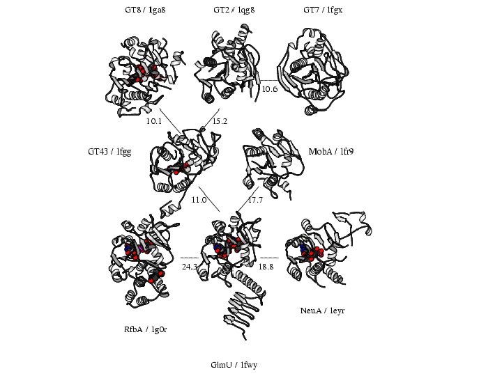
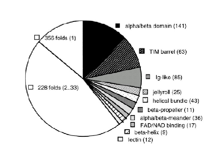
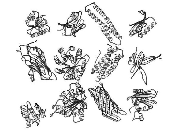
Dali fold space
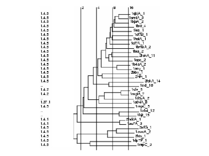
Structure dendrogram • Useful similarity measure groups homologues closer than analogues • Test: manual classification vs. Dali tree
Dali tree approximates evolutionary tree • Topological agreement measured by clustering score – Reference classification: SCOP superfamilies – Find smallest subtree that joins two homologs – Topological distance = fraction of nonhomologs in the subtree • Clustering score = average topological distance over all pairs in a superfamily
Topological distance 12 domains in subtree 6 homologues Topological distance 6 / 12 = 0. 5 Test pair Common subtree Clustering score of green superfamily is 0. 77 Structure similarity
Topogical agreement Dali / SCOP • Average clustering score of Dali similarity tree vs. SCOP superfamilies = 0. 76 • 58 % of 330 SCOP superfamilies (more than one member) occupied ‘pure’ subtree • 96 / 140 split SCOP superfamilies had clustering score < 0. 5, suggesting SCOP unifies dissimilar folds based on nonstructural considerations
Scop – level 1 • 1. 2. 3. Classes: All alpha proteins (151) All beta proteins (111) Alpha and beta proteins (a/b) (117) Mainly parallel beta sheets (beta-alpha-beta units) 4. Alpha and beta proteins (a+b) (212) Mainly antiparallel beta sheets (segregated alpha and beta regions) 5. Multi-domain proteins (alpha and beta) (39) Folds consisting of two or more domains belonging to different classes 6. Membrane and cell surface proteins and peptides (12) Does not include proteins in the immune system 7. Small proteins (59) Usually dominated by metal ligand, heme, and/or disulfide bridges 8. Coiled coil proteins (5) Not a true class 9. Low resolution protein structures (17) Not a true class 10. Peptides (95) Peptides and fragments. Not a true class 11. Designed proteins (36) Experimental structures of proteins with essentially non-natural sequences. Not a true class
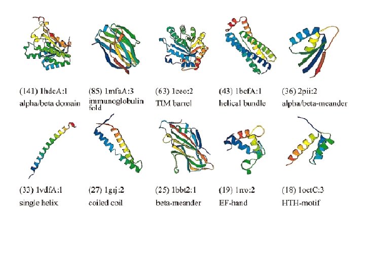
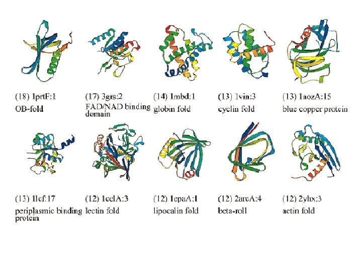
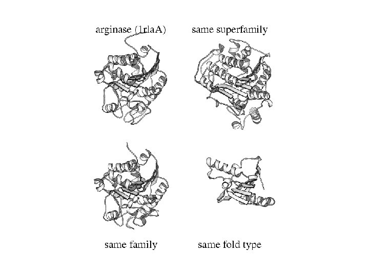
Scop – level 2 • Fold: Major structural similarity • Proteins are defined as having a common fold if they have the same major secondary structures in the same arrangement and with the same topological connections. Different proteins with the same fold often have peripheral elements of secondary structure and turn regions that differ in size and conformation. In some cases, these differing peripheral regions may comprise half the structure. Proteins placed together in the same fold category may not have a common evolutionary origin: the structural similarities could arise just from the physics and chemistry of proteins favoring certain packing arrangements and chain topologies.
Scop – level 3 • Superfamily: Probable common evolutionary origin • Proteins that have low sequence identities, but whose structural and functional features suggest that a common evolutionary origin is probable are placed together in superfamilies. For example, actin, the ATPase domain of the heat shock protein, and hexokinase together form a superfamily.
Scop – level 4 Family: Clear evolutionarily relationship Proteins clustered together into families are clearly evolutionarily related. Generally, this means that pairwise residue identities between the proteins are 30% and greater. However, in some cases similar functions and structures provide definitive evidence of common descent in the absense of high sequence identity; for example, many globins form a family though some members have sequence identities of only 15%.
Scop - opened • 1. All alpha proteins (151) 1. Globin-like (2) core: 6 helices; folded leaf, partly opened 2. Long alpha-hairpin (11) 2 helices; antiparallel hairpin, left-handed twist 3. Type I dockerin domain (1) tandem repeat of two calcium-binding loop-helix motifs, distinct from the EF-hand 4. LEM/SAP He. H motif (4) helix-extended loop-helix; parallel helices 5. Cytochrome c (1) core: 3 helices; folded leaf, opened 6. DNA/RNA-binding 3 -helical bundle (10) core: 3 -helices; bundle, closed or partly opened, right-handed twist; up-and down 7. Ruv. A C-terminal domain-like (6) 3 helices; bundle, right-handed twist 8. Putative DNA-binding domain (1) core: 3 helices; architecture is similar to that of the "winged helix" fold but topology is different 9. Spectrin repeat-like (7) 3 helices; bundle, closed, left-handed twist; up-and-down • …
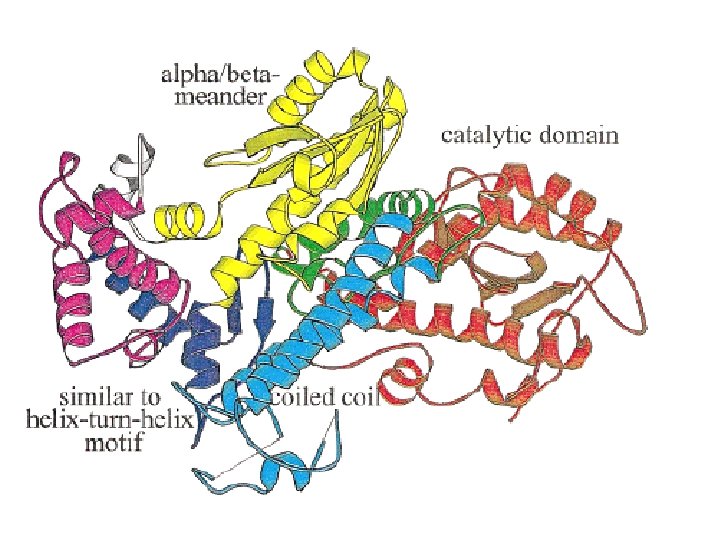
Scop - example • • • Protein: alpha-subunit of urease, catalytic domain from Helicobacter pylori Lineage: Root: scop Class: Alpha and beta proteins (a/b) Mainly parallel beta sheets (beta-alpha-beta units) Fold: TIM beta/alpha-barrel contains parallel beta-sheet barrel, closed; n=8, S=8; strand order 12345678 the first seven superfamilies have similar phosphate-binding sites Superfamily: Metallo-dependent hydrolases the beta-sheet barrel is similarly distorted and capped by a C-terminal helix has transition metal ions bound inside the barrel Family: alpha-subunit of urease, catalytic domain Protein: alpha-subunit of urease, catalytic domain Species: Helicobacter pylori
Scop - example • • 3. Alpha and beta proteins (a/b) (117) Mainly parallel beta sheets (beta-alpha-beta units) 3. 1. TIM beta/alpha-barrel (25) contains parallel beta-sheet barrel, closed; n=8, S=8; strand order 12345678 the first seven superfamilies have similar phosphate-binding sites 1. 2. 3. 4. 5. 6. Triosephosphate isomerase (TIM) (1) Ribulose-phoshate binding barrel (4) Thiamin phosphate synthase (1) Pyridoxine 5'-phosphate synthase (1) FMN-linked oxidoreductases (1) Inosine monophosphate dehydrogenase (IMPDH) (1) The phosphape moiety of substrate binds in the 'common' phosphate-binding site 7. PLP-binding barrel (2) circular permutation of the canonical fold: begins with an alpha helix and ends with a betastrand 8. NAD(P)-linked oxidoreductase (1) 9. (Trans)glycosidases (9) 10. Metallo-dependent hydrolases (8) the beta-sheet barrel is similarly distorted and capped by a C-terminal helix has transition metal ions bound inside the barrel
Scop - nucleotide-binding folds • 3. 2. NAD(P)-binding Rossmann-fold domains (1) core: 3 layers, a/b/a; parallel beta-sheet of 6 strands, order 321456 The nucleotide-binding modes of this and the next two folds/superfamilies are similar – NAD(P)-binding Rossmann-fold domains (11) • 3. 3. FAD/NAD(P)-binding domain (1) core: 3 layers, b/b/a; central parallel beta-sheet of 5 strands, order 32145; top antiparallel beta-sheet of 3 strands, meander – FAD/NAD(P)-binding domain (5) • 3. 4. Nucleotide-binding domain (1) 3 layers: a/b/a; parallel beta-sheet of 5 strands, order 32145; Rossmann-like – Nucleotide-binding domain (3) this superfamily shares the common nucleotide-binding site with and provides a link between the Rossmann-fold NAD(P)-binding and FAD/NAD(P)-binding domains
CATH hierarchy
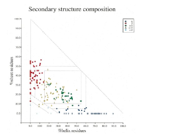
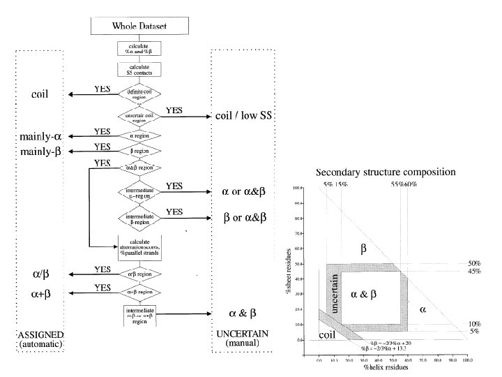
Class, C-level • Class is determined according to the secondary structure composition and packing within the structure. It can be assigned automatically for over 90% of the known structures using the method of Michie et al. (1996). For the remainder, manual inspection is used and where necessary information from the literature taken into account. Three major classes are recognised; mainlyalpha, mainly-beta and alpha-beta. This last class (alphabeta) includes both alternating alpha/beta structures and alpha+beta structures, as originally defined by Levitt and Chothia (1976). A fourth class is also identified which contains protein domains which have low secondary structure content.
SSAP space
Dali space
Architecture, A-level • This describes the overall shape of the domain structure as determined by the orientations of the secondary structures but ignores the connectivity between the secondary structures. It is currently assigned manually using a simple description of the secondary structure arrangement e. g. barrel or 3 -layer sandwich. Reference is made to the literature for well-known architectures (e. g the beta-propellor or alpha four helix bundle). Procedures are being developed for automating this step.
Topology (Fold family), T-level • Structures are grouped into fold families at this level depending on both the overall shape and connectivity of the secondary structures. This is done using the structure comparison algorithm SSAP (Taylor & Orengo (1989)). Parameters for clustering domains into the same fold family have been determined by empirical trials throughout the databank (Orengo et al. (1992), Orengo et al. (1993)). Structures which have a SSAP score of 70 and where at least 60% of the larger protein matches the smaller protein are assigned to the same T level or fold family.
T-level - exceptions • Some fold families are very highly populated (Orengo et al. (1994)) particularly within the mainly-beta 2 -layer sandwich architectures and the alpha-beta 3 -layer sandwich architectures. In order to appreciate the structural relationships within these families more easily, they are currently subdivided using a higher cutoff on the SSAP score (75 for some mainly-beta and alphabeta families, 80 for some mainly-alpha families, together with a higher overlap requirement (70%)).
Homologous Superfamily, H-level • This level groups together protein domains which are thought to share a common ancestor and can therefore be described as homologous. Similarities are identified first by sequence comparisons and subsequently by structure comparison using SSAP. Structures are clustered into the same homologous superfamily if they satisfy one of the following criteria: – Sequence identity >= 35%, 60% of larger structure equivalent to smaller – SSAP score >= 80. 0 and sequence identity >= 20% 60% of larger structure equivalent to smaller – SSAP score >= 80. 0, 60% of larger structure equivalent to smaller, and domains which have related functions
Sequence families, S-level • Structures within each H-level are further clustered on sequence identity. Domains clustered in the same sequence families have sequence identities >35% (with at least 60% of the larger domain equivalent to the smaller), indicating highly similar structures and functions.
Arkkitehtuuri
Mainly alpha Up-down bundle Horseshoe Orthogonal bundle Solenoid
Mainly beta Ribbon Roll Single sheet Barrel
Clam Distorted sandwich 3 -layer sandwich Sandwich
Prism Aligned prism Trefoil
6 -propellor 5 -propellor 7 -propellor 4 -propellor
8 -propellor Complex 2 -solenoid 3 -solenoid
Mixed alpha-beta Roll Super roll Barrel Horseshoe
2 -layer sandwich 3 -layer bba sandwich 3 -layer aba sandwich 4 -layer sandwich
Alpha-beta prism Box Complex (Immunoglobulin/ Lipoprotein) 5 -stranded propeller
Complex (mixed alpha-beta) Irregular
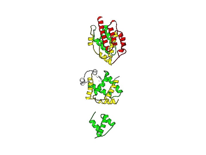
Yhteenveto - arkkitehtuuri • arkkitehtuuri = sekundaarirakenteiden yhteen pakkaaminen – silmukoiden kiinnittyminen (topologia) jätetty huomiotta • suositut arkkitehtuurit muistuttavat säännöllisiä geometrisia tiiveimpiä pakkauksia • konvergentti evoluutio samanlaisiin laskoksiin – Rakenne säilyy vaikka sekvenssit muuntelevat paljonkin – antaa evoluutiolle pelitilaa • Hajautettu koodi: joistakin proteiineista on muutettu 30 % aminohapoista alaniiniksi laskoksen muuttumatta
Evidence of common ancestry? • Conservation of unusual structural features • Clusters of conserved residues – giving especially sharp signatures in enzyme active sites • Sequence similarity through bridging intermediates – leading to elongated clusters in protein space • Functional similarities – conserved molecular protocols • Proteins with clear sequence similarity are grouped into families. • Pairs of proteins in the same superfamily but different families comprise a popular benchmark for testing the ability of computational methods to identify remote homology.
Aminohappojen ominaisuuksia