STT 592 002 Intro to Statistical Learning REVIEW

STT 592 -002: Intro. to Statistical Learning REVIEW: LINEAR REGRESSION Chapter 03 Disclaimer: This PPT is modified based on IOM 530: Intro. to Statistical Learning "Some of the figures in this presentation are taken from "An Introduction to Statistical Learning, with applications in R" (Springer, 2013) with permission from the authors: G. James, D. Witten, T. Hastie and R. Tibshirani " 1

STT 592 -002: Intro. to Statistical Learning Outline ØLinear Regression Model ØSimple Linear, Multivariate Linear ØLeast Squares Fit ØMeasures of Fit ØInference in Regression ØOther Considerations in Regression Model ØQualitative Predictors ØInteraction Terms ØNon-Linear Regression Model ØPotential Fit Problems ØLinear vs. KNN Regression 2

STT 592 -002: Intro. to Statistical Learning 3 Statistics synonyms • Depending on the context, an independent variable is sometimes called a "predictor variable", regressor, covariate, "controlled variable", "manipulated variable", "explanatory variable", exposure variable (see reliability theory), "risk factor" (see medical statistics), "feature" (in machine learning and pattern recognition) or "input variable. "[9][10] In econometrics, the term "control variable" is usually used instead of "covariate". [11][12][13][14][15] • Depending on the context, a dependent variable is sometimes called a "response variable", "regressand", "criterion", "predicted variable", "measured variable", "explained variable", "experimental variable", "responding variable", "outcome variable", "output variable" or "label". [10] https: //en. wikipedia. org/wiki/Dependent_and_independent_variables

STT 592 -002: Intro. to Statistical Learning Case 1: Advertisement Data Advertising=read. csv("http: //faculty. marshall. usc. edu/garethjames/ISL/Advertising. csv", header=TRUE); newdata=Advertising[, -1] fix(newdata) View(newdata) names(newdata) pairs(newdata) cor(newdata[ , 2: 4]) 4

STT 592 -002: Intro. to Statistical Learning cor(newdata) cor(newdata[ , 2: 4]) 5

STT 592 -002: Intro. to Statistical Learning Advertisement Data: background 6

STT 592 -002: Intro. to Statistical Learning 7 Advertisement Data: • 1. Is there a relationship b/w advertising budget (TV, Radio, or Newspaper) and sales? • 2. How strong is relationship b/w advertising budget (TV, Radio, or Newspaper) and sales? • 3. Which media contribute to sales?

STT 592 -002: Intro. to Statistical Learning 8 Advertisement Data: • 4. How accurately can we estimate effect of each medium on sales? • 5. How accurately can we predict future sales? • 6. Is the relationship linear? • 7. Is there synergy among advertising media?

Correlation tells us about strength (scatter) and direction of the linear relationship between two quantitative variables. In addition, we would like to have a numerical description of how both variables vary together. For instance, is one variable increasing faster than the other one? And we would like to make predictions based on that numerical description. But which line best describes our data?

10 Simple linear regression model •

The least-squares regression line Error=observed value – predicted value. The least-squares regression line is the unique line such that the sum of the squared vertical (y) distances between the data points and the line is the smallest possible. Distances between the points and line are squared so all are positive values. This is done so that distances can be properly added (Pythagoras).

STT 592 -002: Intro. to Statistical Learning 12 Advertisement Data: how to fit the data? LSE

STT 592 -002: Intro. to Statistical Learning 13 Simple Linear Regression: LSE background

STT 592 -002: Intro. to Statistical Learning 14 Simple Linear Regression: LSE background

STT 592 -002: Intro. to Statistical Learning 15 Simple Linear Regression: LSE background t-statistic ~t(n-2)

STT 592 -002: Intro. to Statistical Learning 16 Degree of Freedom of Linear regression • Each sum of squares (SSE) has a corresponding degrees of • • • freedom (df) associated with it. Total df is n-1, one less than the number of observations. The Regression df is the number of independent variables in the model. For simple linear regression (only one x), the Regression df is 1. The Error df is the difference between the Total df and the Regression df. For simple linear regression, the residual df is n 2. Or: Notice that to obtain �� 1 -hat, we require an estimate of two quantities: μx, and μy, which we have in �� -bar and �� -bar. We lose a degree of freedom for each of these estimates.

STT 592 -002: Intro. to Statistical Learning 17 Advertisement Data for simple linear regression Advertising=read. csv("http: //faculty. marshall. usc. edu/garethjames/ISL/Advertising. csv", header=TRUE); lm. fit=lm(sales~TV, data=Advertising) ## to get Table 3. 1 summary(lm. fit) names(lm. fit) coef(lm. fit) confint(lm. fit)

STT 592 -002: Intro. to Statistical Learning 18 Q: Is b 1=0 i. e. is X an important variable? ØWe use a hypothesis test to answer this question Ø H 0: 1=0 vs Ha: 1 0 ØCalculate Number of standard deviations away from zero. ØIf t is large (equivalently p-value is small) we can be sure that j 0 and that there is a relationship is 17. 67 SE’s from 0 P-value

STT 592 -002: Intro. to Statistical Learning 19 Measures of Fit: R 2 ØSome of the variation in Y can be explained by variation in the X’s and some cannot. Ø R 2 tells you the % of variance that can be explained by the regression on X. R 2 is always between 0 and 1. Zero means no variance has been explained. One means it has all been explained (perfect fit to the data).

STT 592 -002: Intro. to Statistical Learning 20 Multiple Linear Regression Model ØY: Quantitative Response; Xj: j-th predictor ØThe parameters in the linear regression model are very easy to interpret. Ø 0 is the intercept (i. e. the average value for Y if all the X’s are zero), j is the slope for the jth variable Xj Ø j is the average increase in Y when Xj is increased by one unit and all other X’s are held constant.

STT 592 -002: Intro. to Statistical Learning Least Squares Estimate ØWe estimate the parameters using least squares i. e. minimize 21

STT 592 -002: Intro. to Statistical Learning 22 Relationship between population and least squares lines Population line Least Squares line Ø We would like to know 0 through p i. e. the population line. Instead we know through i. e. the least squares line. Ø Hence we use through as guesses for 0 through p and as a guess for Yi. The guesses will not be perfect just as is not a perfect guess for .

23 STT 592 -002: Intro. to Statistical Learning Inference in Regression Estimated (least squares) line. ØThe regression line from the 14 sample is not the regression line from the population. ØWhat we want to do: Ø Ø Ø 12 10 Assess how well the line describes the plot. Guess the slope of the population line. Guess what value Y would take for a given X value 8 6 4 2 0 -10 -5 0 X 5 10 True (population) line. Unobserved

STT 592 -002: Intro. to Statistical Learning 24 Some Relevant Questions 1. Is j=0 or not? We can use a hypothesis test to answer this question. If we can’t be sure that j≠ 0 then there is no point in using Xj as one of our predictors. 2. Can we be sure that at least one of our X variables is a useful predictor i. e. is it the case that β 1= β 2= = β p=0?

STT 592 -002: Intro. to Statistical Learning 25 Advertisement Data for multiple linear regression ## To get Table 3. 4 ## Advertising=read. csv("http: //faculty. marshall. usc. edu/garethjames/ISL/Advertising. csv", header=TRUE); lm. fit=lm(sales~TV+radio+newspaper, data=Advertising) summary(lm. fit) names(lm. fit) coef(lm. fit) confint(lm. fit)

STT 592 -002: Intro. to Statistical Learning 26 1. Is bj=0 i. e. is Xj an important variable? ØWe use a hypothesis test to answer this question Ø H 0: j=0 vs Ha: j 0 ØCalculate Number of standard deviations away from zero. ØIf t is large (equivalently p-value is small) we can be sure that j 0 and that there is a relationship is 17. 67 SE’s from 0 P-value

STT 592 -002: Intro. to Statistical Learning 27 Testing Individual Variables Is there a (statistically detectable) linear relationship between Newspapers and Sales after all the other variables have been accounted for? No: big p-value Small p-value in simple regression Almost all the explaining that Newspapers could do in simple regression has already been done by TV and Radio in multiple regression!

STT 592 -002: Intro. to Statistical Learning 28 Multiple Linear Regression: LSE background Q: how to find p-value? Q: ANOVA? =(MSmodel)/(MSerror)

STT 592 -002: Intro. to Statistical Learning 29 2. Is the whole regression explaining anything at all? ØTest for: • H 0: all slopes = 0 ( 1= 2= = p=0), • Ha: at least one slope 0 Answer comes from the F test in the ANOVA (ANalysis Of VAriance) table. The ANOVA table has many pieces of information. What we care about is the F Ratio and the corresponding p-value.

STT 592 -002: Intro. to Statistical Learning 30 Multiple Linear Regression: LSE background Here we go…

STT 592 -002: Intro. to Statistical Learning 31 Adjusted R-Square • R-square will always increase when more variables are added to the model, even if those variables are only weakly associated with the response. This is due to the fact that adding another variable to the least squares equations must allow us to fit the training data (though not necessarily the testing data) more accurately.

STT 592 -002: Intro. to Statistical Learning 32 Deciding on Important Variables: variable selection ## To get Table 3. 4 ## Advertising=read. csv("http: //faculty. marshall. usc. edu/garethjames/ISL/Advertising. csv", header=TRUE); lm. fit 1=lm(sales~newspaper, data=Advertising) summary(lm. fit 1) lm. fit 2=lm(sales~newspaper+TV, data=Advertising) summary(lm. fit 2) lm. fit 3=lm(sales~newspaper+TV+radio, data=Advertising) summary(lm. fit 3) lm. fit 4=lm(sales~TV+radio, data=Advertising) summary(lm. fit 4)

STT 592 -002: Intro. to Statistical Learning 33 Assumptions for linear regression • Linearity: The relationship between X and the mean of Y is linear. • Homoscedasticity: The variance of residual is the same for any value of X. • Independence: Observations are independent of each other. • Normality: For any fixed value of X, Y is normally distributed.

STT 592 -002: Intro. to Statistical Learning 34 Model fits • Should check if the model works well for data. . . in many different ways. • We pay great attention to regression results, such as slope coefficients, p-values, or R 2 that tell us how well a model represents given data. That’s not the whole picture though. • Adjusted R-square; • RSE; • Plot the data to detect any synergy or interaction effect. https: //data. library. virginia. edu/diagnostic-plots/

STT 592 -002: Intro. to Statistical Learning 35 Understanding diagnostic plots for linear regression analysis • Reference website: • https: //data. library. virginia. edu/diagnostic-plots/ • https: //www. andrew. cmu. edu/user/achoulde/94842/homework/regress ion_diagnostics. html • http: //analyticspro. org/2016/03/07/r-tutorial-how-to-use-diagnostic- plots-for-regression-models/

STT 592 -002: Intro. to Statistical Learning 36 Understanding diagnostic plots for linear regression analysis • Residuals could show poorly a model represents data. • Residuals are leftover of the outcome variable after fitting a model (predictors) to data and they could reveal unexplained patterns in the data by the fitted model. • Using this information, not only could you check if linear regression assumptions are met, but you could improve your model in an exploratory way. https: //data. library. virginia. edu/diagnostic-plots/

STT 592 -002: Intro. to Statistical Learning 37 Understanding diagnostic plots for linear regression analysis • Built-in diagnostic plots for linear regression analysis in R Eg: data(women) # Load a built-in data called ‘women’ fit = lm(weight ~ height, women) # Run a regression analysis par(mfrow=c(2, 2)) # Change the panel layout to 2 x 2 plot(fit) ## linear model of “fit” par(mfrow=c(1, 1)) # Change back to 1 x 1 You will often see numbers next to some points in each plot. They are extreme values based on each criterion and identified by the row numbers in the data set. https: //data. library. virginia. edu/diagnostic-plots/

STT 592 -002: Intro. to Statistical Learning 1. Residuals vs Fitted plot https: //data. library. virginia. edu/diagnostic-plots/ 38

STT 592 -002: Intro. to Statistical Learning 39 1. Residuals vs Fitted plot • Check if residuals have non-linear patterns or not. • Equally spread residuals around a horizontal line without distinct patterns • a good indication for linear relationships. • Diagnostics 1: • No distinctive pattern in Case 1, • A parabola pattern in Case 2, where the non-linear relationship was not explained by the model and was left out in the residuals. https: //data. library. virginia. edu/diagnostic-plots/

STT 592 -002: Intro. to Statistical Learning 2. Normal Q-Q Plot https: //data. library. virginia. edu/diagnostic-plots/ 40

STT 592 -002: Intro. to Statistical Learning 41 2. Normal Q-Q Plot • To check if residuals are normally distributed. • Do residuals follow a straight line well or do they deviate severely? It’s good if residuals are lined well on the straight dashed line (normally distributed). • Diagnostics 2: • Of course they wouldn’t be a perfect straight line and this will be your call. • Case 2 shows definitely some concerns. • Not too much concerns on Case 1, although observation #38 looks a little off. Keep in mind that #38 might be a potential problem. • For more detailed information, see Understanding Q-Q plots. https: //data. library. virginia. edu/understanding-q-q-plots/

STT 592 -002: Intro. to Statistical Learning 3. Scale-Location Plot https: //data. library. virginia. edu/diagnostic-plots/ 42

STT 592 -002: Intro. to Statistical Learning 43 3. Scale-Location Plot, or Spread-Location plot • It shows if residuals are spread equally along the ranges of predictors. • To check the assumption of equal variance (homoscedasticity). It’s good if you see a horizontal line with equally (randomly) spread points. • Diagnostics 3 • Case 1: the residuals appear randomly spread. • Whereas, in Case 2, the residuals begin to spread wider along the x-axis as it passes around 5. Because the residuals spread wider and wider, the red smooth line is not horizontal and shows a steep angle in Case 2. https: //data. library. virginia. edu/diagnostic-plots/

STT 592 -002: Intro. to Statistical Learning 44 4. Residuals vs Leverage Plot • Influence : The Influence of an observation can be thought of in terms of how much the predicted scores would change if the observation is excluded. Cook’s Distance is a pretty good measure of influence of an observation. • Leverage : The leverage of an observation is based on how much the observation’s value on the predictor variable differs from the mean of the predictor variable. The more the leverage of an observation, the greater potential that point has in terms of influence. http: //analyticspro. org/2016/03/07/r-tutorial-how-to-use-diagnostic-plots-for-regression-models/

Review: STT 215: Outliers and influential points Outlier: observation that lies outside the overall pattern of observations. “Influential individual”: observation that markedly changes the regression if removed. This is often an outlier on the x-axis. Child 19 = outlier in y direction Child 19 is an outlier of the relationship. Child 18 is only an outlier in the x direction and thus might be an influential point. Child 18 = outlier in x direction

Review: STT 215: Outliers and influential points outlier in y -direction All data Without child 18 Without child 19 Are these points influential? From previous slide: 1) Obs. #19 with Influence low and leverage low; 2) Obs. #18 with Influence high and leverage high influential

STT 592 -002: Intro. to Statistical Learning 47 http: //sphweb. bumc. bu. edu/otlt/MPHModules/BS/R/R 5_Correlation. Regression/R 5_Correlation-Regression 7. html From previous slide: 1) Obs. #19 with Influence low and leverage low; 2) Obs. #18 with Influence high and leverage high • Outliers: An observation that has a large residual, i. e. , observed value is very different from that predicted by the regression model. • Leverage points: A leverage point is an observation that has a value of x that is far away from the mean of x. • Influential observations: An influential observation is defined as an observation that changes the slope of the line. Thus, influential points have a large influence on the fit of the model. One method to find influential points is to compare the fit of the model with and without each observation.

STT 592 -002: Intro. to Statistical Learning 4. Residuals vs Leverage Plot https: //data. library. virginia. edu/diagnostic-plots/ 48

STT 592 -002: Intro. to Statistical Learning 49 4. Residuals vs Leverage Plot • To check if any influential cases. • Some cases could be extreme cases against a regression line and can alter the results if we exclude them from analysis. • Watch out for outlying values at the upper right corner or at the lower right corner. Those spots are the places where cases can be influential against a regression line. • Look for cases outside of a dashed line, Cook’s distance. When cases are outside of the Cook’s distance (dotted red lines), the cases are influential to the regression results. • The regression results will be altered if we exclude those cases. https: //data. library. virginia. edu/diagnostic-plots/

STT 592 -002: Intro. to Statistical Learning 50 4. Residuals vs Leverage Plot • Case 1: Typical look when there is no influential case(s). You can barely see Cook’s distance lines (a red dashed line) because all cases are well inside of the Cook’s distance lines. • Case 2: a case is far beyond the Cook’s distance lines (the other residuals appear clustered on the left because the second plot is scaled to show larger area than the first plot). • The plot identified the influential observation as #49. If #49 is excluded, the slope coefficient changes from 2. 14 to 2. 68 and R 2 from. 757 to. 851. Pretty big impact! https: //data. library. virginia. edu/diagnostic-plots/

STT 592 -002: Intro. to Statistical Learning 51 4. With high Leverage observations • In this case observation #49 has high leverage and we have 3 choices • Choice 1: Justify the inclusion of #49 and keep model as is • Choice 2 : Include quadratic term as indicated by Residual vs fitted plot and remodel • Choice 3: Exclude observation #49 and remodel.

STT 592 -002: Intro. to Statistical Learning 52 Understanding diagnostic plots for linear regression analysis • Residuals could show poorly a model represents data. • Residuals are leftover of the outcome variable after fitting a model (predictors) to data and they could reveal unexplained patterns in the data by the fitted model. • Using this information, not only could you check if linear regression assumptions are met, but you could improve your model in an exploratory way. • Summary: • Four plots show potential problematic cases with the row numbers of the data in the dataset. If some cases are identified across all four plots, you might want to take a close look at them individually. Is there anything special for the subject? Or could it be simply errors in data entry? https: //data. library. virginia. edu/diagnostic-plots/

STT 592 -002: Intro. to Statistical Learning 53 Example: Model fits for Advertising data • Residual Plots Advertising=read. csv("http: //faculty. marshall. usc. edu/garethjames/ISL/Advertising. csv", header=TRUE); lm. fit=lm(sales~TV+radio+newspaper, data=Advertising) par(mfrow=c(2, 2)) plot(lm. fit) plot(predict(lm. fit), residuals(lm. fit)) plot(predict(lm. fit), rstudent(lm. fit)) plot(hatvalues(lm. fit)) which. max(hatvalues(lm. fit))

STT 592 -002: Intro. to Statistical Learning Example: Advertising data 54

STT 592 -002: Intro. to Statistical Learning Outline ØThe Linear Regression Model ØLeast Squares Fit ØMeasures of Fit ØInference in Regression ØOther Considerations in Regression Model ØQualitative Predictors ØInteraction Terms ØPotential Fit Problems ØLinear vs. KNN Regression 55

STT 592 -002: Intro. to Statistical Learning 56 Credit Data: Credit=read. csv("http: //www-bcf. usc. edu/~gareth/ISL/Credit. csv", header=TRUE); head(Credit); newdata=Credit [, -1] fix(newdata); names(newdata) pairs(newdata[, c(1, 2, 4, 5, 6, 7)])

STT 592 -002: Intro. to Statistical Learning Credit Data: Credit=read. csv("http: //faculty. marshall. usc. edu/garethjames/ISL/Credit. csv", header=TRUE); head(Credit); newdata=Credit [, -1] fix(newdata); names(newdata) pairs(newdata[, c(1, 2, 4, 5, 6, 7)]) Q: Numerical/Quantitative Variables? Q: Categorical/Qualitative Variables? 57

STT 592 -002: Intro. to Statistical Learning 58 Qualitative Predictors ØHow do you stick “gender” with “men” and “women” (category listings) into a regression equation? ØCode them as indicator variables (dummy variables) ØFor example we can “code” Males=0 and Females= 1.

STT 592 -002: Intro. to Statistical Learning 59 One qualitative predictor with two levels • Q: To investigate differences in credit card balance between males and females, ignoring the other variables for the moment. ØTwo genders (male and female). Let Øthen the regression equation is

STT 592 -002: Intro. to Statistical Learning Credit Data: Credit=read. csv("http: //faculty. marshall. usc. edu/garethjames/ISL/Credit. csv", header=TRUE); lm. fit=lm(Balance~Gender, data=Credit) summary(lm. fit); contrasts(Credit$Gender) 60

STT 592 -002: Intro. to Statistical Learning 61 Two qualitative predictors with only two levels ØY: Balance. We want to include income and gender. ØTwo genders (male and female). Let Øthen the regression equation is Ø 2 is the average extra balance each month that females have for given income level. Males are the “baseline”.

STT 592 -002: Intro. to Statistical Learning 62 Other Coding Schemes ØThere are different ways to code categorical variables. ØTwo genders (male and female). Let Øthen the regression equation is Ø 2 is the average amount that females are above the average, for any given income level. 2 is also the average amount that males are below the average, for any given income level.

STT 592 -002: Intro. to Statistical Learning 63 One qualitative predictor with more than two levels • Q: To investigate differences in credit card balance between Ethnicity, ignoring the other variables for the moment. contrasts(Credit$Ethnicity) ØThree levels of Ethnicity

STT 592 -002: Intro. to Statistical Learning 64 Credit Data: Credit=read. csv("http: //faculty. marshall. usc. edu/garethjames/ISL/Credit. csv", header=TRUE); lm. fit=lm(Balance~Ethnicity, data=Credit) contrasts(Credit$Ethnicity) summary(lm. fit)

STT 592 -002: Intro. to Statistical Learning Other Issues Discussed ØInteraction terms ØNon-linear effects ØCollinearity and Multicollinearity ØModel Selection 65

STT 592 -002: Intro. to Statistical Learning 66 Interaction ØWhen the effect on Y of increasing X 1 depends on another X 2. [synergy effect] ØExample #1: Ø# of Shark attack (Y), to ice cream sales(X 1) & temperature (X 2)? ØExample #2: Advertising Data: Ø TV and radio advertising both increase sales. Ø Perhaps spending money on both of them may increase sales more than spending the same amount on one alone? ØExample #3: Ø Maybe the effect on Salary (Y) when increasing Position (X 1) depends on gender (X 2)? Ø For example maybe Male salaries go up faster (or slower) than Females as they get promoted.

STT 592 -002: Intro. to Statistical Learning 67 Interaction in advertising Ø Spending $1 extra on TV increases average sales by 0. 0191 + 0. 0011 Radio Ø Spending $1 extra on Radio increases average sales by 0. 0289 + 0. 0011 TV Interaction Term

STT 592 -002: Intro. to Statistical Learning Credit Data: Advertising=read. csv("http: //faculty. marshall. usc. edu/garethjames/ISL/Advertising. csv", header=TRUE); lm. fit=lm(sales~TV*radio, data=Advertising) summary(lm. fit) 68

STT 592 -002: Intro. to Statistical Learning 69 Parallel Regression Lines Line for women Regression equation female: salary = 112. 77+1. 86 + 6. 05 position males: salary = 112. 77 -1. 86 + 6. 05 position Different intercepts Same slopes Line for men Parallel lines have the same slope. Dummy variables give lines different intercepts, but their slopes are still the same.

STT 592 -002: Intro. to Statistical Learning 70 Interaction Effects ØOur model has forced the line for men and the line for women to be parallel. ØParallel lines say that promotions have the same salary benefit for men as for women. ØIf lines aren’t parallel then promotions affect men’s and women’s salaries differently.

71 STT 592 -002: Intro. to Statistical Learning Should the Lines be Parallel? 170 160 150 140 130 120 110 0 1 2 3 4 5 6 7 8 9 10 Position Interaction is not significant Interaction between gender and position

STT 592 -002: Intro. to Statistical Learning 72 Collinearity and Multicollinearity ØTo detect collinearity: Use Correlation matrix of predictors. ØAn element in matrix with a large absolute value indicates a pair of highly correlated variables, and therefore a collinearity problem in the data. ØBut not all collinearity problems can be detected by inspection of the correlation matrix. ØMulticollinearity: collinearity to exist between three or more variables, even if no pair of variables has a particularly high correlation. ØFor multicollinearity, compute the variance inflation factor (VIF).

STT 592 -002: Intro. to Statistical Learning 73 Collinearity and Multicollinearity ØFor multicollinearity, compute the variance inflation factor (VIF). ØVIF≥ 1. ØAs a rule of thumb, a VIF value that exceeds 5 or 10 indicates a problematic amount of collinearity. Ø

STT 592 -002: Intro. to Statistical Learning Calculate VIF • https: //en. wikipedia. org/wiki/Variance_inflation_factor vif(lm(y~x, data)) 74

STT 592 -002: Intro. to Statistical Learning 75 Collinearity and Multicollinearity ØTo solve for collinearity: Ø 1) Drop one of the problematic variables from the regression. Ø 2) Combine the collinear variables together into a single predictor. ØFor instance, we might take the average of standardized versions of those two variables to create a new variable.

STT 592 -002: Intro. to Statistical Learning Outline ØThe Linear Regression Model ØLeast Squares Fit ØMeasures of Fit ØInference in Regression ØOther Considerations in Regression Model ØQualitative Predictors ØInteraction Terms ØPotential Fit Problems ØLinear vs. KNN Regression 76

STT 592 -002: Intro. to Statistical Learning Potential Fit Problems There a number of possible problems that one may encounter when fitting the linear regression model. 1. Non-linearity of the data [residual plot] 2. Dependence of the error terms 3. Non-constant variance of error terms 4. Outliers 5. High leverage points 6. Collinearity See Section 3. 3. 3 for more details. 77

STT 592 -002: Intro. to Statistical Learning Outline ØThe Linear Regression Model ØLeast Squares Fit ØMeasures of Fit ØInference in Regression ØOther Considerations in Regression Model ØQualitative Predictors ØInteraction Terms ØPotential Fit Problems ØLinear vs. KNN Regression 78

STT 592 -002: Intro. to Statistical Learning 79 K-Nearest Neighbors (KNN) classifier (Sec 2. 2) • Given a positive integer K and a test observation x 0, the KNN classifier first identifies the neighbors K points in the training data that are closest to x 0, represented by N 0. • It then estimates the conditional probability for class j as the fraction of points in N 0 whose response values equal j: • Finally, KNN applies Bayes rule and classifies the test observation x 0 to the class with the largest probability.

STT 592 -002: Intro. to Statistical Learning 80 K-Nearest Neighbors (KNN) classifier (Sec 2. 2) • A small training data set: 6 blue and 6 orange observations. • Goal: to make a prediction for the black cross. Consider K=3. • KNN identify 3 observations that are closest to the cross. This neighborhood is shown as a circle. It consists of 2 blue points and 1 orange point, resulting in estimated probabilities of 2/3 for blue class and 1/3 for the orange class. • KNN predict that the black cross belongs to the blue class.

STT 592 -002: Intro. to Statistical Learning 81 KNN Regression Øk. NN Regression is similar to the k. NN classifier. ØTo predict Y for a given value of X, consider k closest points to X in training data and take the average of the responses. i. e. ØIf k is small, k. NN is much more flexible than linear regression. ØIs that better?

STT 592 -002: Intro. to Statistical Learning KNN Fits for k =1 and k = 9 82

STT 592 -002: Intro. to Statistical Learning 83 KNN Fits in One Dimension (k =1 and k = 9)

STT 592 -002: Intro. to Statistical Learning Linear Regression Fit 84

STT 592 -002: Intro. to Statistical Learning KNN vs. Linear Regression 85

STT 592 -002: Intro. to Statistical Learning Not So Good in High Dimensional Situations 86

STT 592 -002: Intro. to Statistical Learning 87 R Lab in Chap 3 • Let’s work on the R lab in Chap 3. Here are some key points in the R Lab: • summary(lm. fit)$r. sq R 2, • summary(lm. fit)$sigma RSE. • vif() to compute variance inflation factors

STT 592 -002: Intro. to Statistical Learning 89 THE BIAS-VARIANCE TRADE -OFF Let’s Go back to Chapter 02: Statistical Learning

WHERE DOES THE ERROR COME FROM? Disclaimer: This PPT is modified based on Dr. Hung-yi Lee http: //speech. ee. ntu. edu. tw/~tlkagk/courses_ML 17. ht ml

Estimator Bias + Variance

Bias and Variance of Estimator • unbiased

Bias and Variance of Estimator unbiased • Smaller N Larger N Variance depends on the number of samples

Bias and Variance of Estimator • Increase N Biased estimator

Varianc e Bias

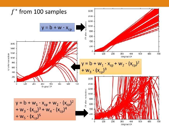
Variance Small Variance Large Variance Simpler model is less influenced by the sampled data Consider the extreme case f(x) of degree

Bias • Larg e Bias Small Bias

Degree=1 Degree=5 Degree=3

Bias model Larg e Bias model Small Bias

What to do with large bias? • Diagnosis: • If your model cannot even fit the training examples, then you have large bias Underfitting • If you can fit the training data, but large error on testing data, then you probably have large Overfitting variance • For bias, redesign your model: • Add more features as input • A more complex model large bias

What to do with large variance? • More data Very effective, but not always • practical Regularization 10 examples May increase bias 100 examples

Bias v. s. Variance Error from bias Error from variance Error observed Overfitting Underfitting Horizontal Axis: Model Complex Large Bias Small Variance Small Bias Large Variance

Consequently… Average Error on Testing Data error due to "bias" and error due to "variance" A more complex model does not always lead to better performance on testing data.

Cross Validation public Training Set Validation set Testing Set private Testing Set Model 1 Err = 0. 9 Using the results of public testing data to tune your model You are making public set better than private set. Model 2 Err = 0. 7 Not recommend Model 3 Err = 0. 5 Err > 0. 5

N-fold Cross Validation Training Set Model 1 Model 2 Model 3 Train Val Err = 0. 2 Err = 0. 4 Train Val Train Err = 0. 4 Err = 0. 5 Val Train Err = 0. 3 Err = 0. 6 Err = 0. 3 Avg Err = 0. 3 = 0. 5 = 0. 4 Testing Set public Testing Set private