ICS 178 Intro Machine Learning decision trees random

ICS 178 Intro Machine Learning decision trees, random forests, bagging, boosting.

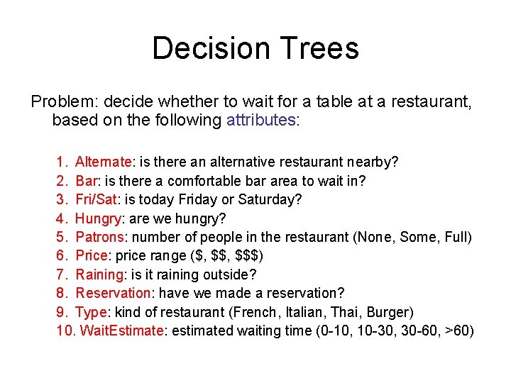
Decision Trees Problem: decide whether to wait for a table at a restaurant, based on the following attributes: 1. Alternate: is there an alternative restaurant nearby? 2. Bar: is there a comfortable bar area to wait in? 3. Fri/Sat: is today Friday or Saturday? 4. Hungry: are we hungry? 5. Patrons: number of people in the restaurant (None, Some, Full) 6. Price: price range ($, $$$) 7. Raining: is it raining outside? 8. Reservation: have we made a reservation? 9. Type: kind of restaurant (French, Italian, Thai, Burger) 10. Wait. Estimate: estimated waiting time (0 -10, 10 -30, 30 -60, >60)

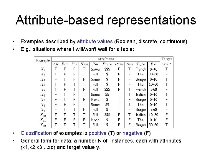
Attribute-based representations • • Examples described by attribute values (Boolean, discrete, continuous) E. g. , situations where I will/won't wait for a table: • • Classification of examples is positive (T) or negative (F) General form for data: a number N of instances, each with attributes (x 1, x 2, x 3, . . . xd) and target value y.

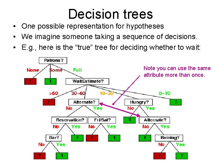
Decision trees • One possible representation for hypotheses • We imagine someone taking a sequence of decisions. • E. g. , here is the “true” tree for deciding whether to wait: Note you can use the same attribute more than once.

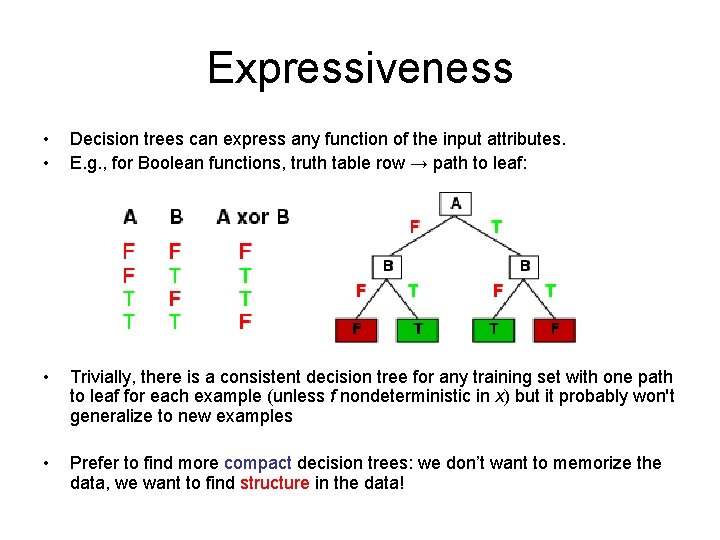
Expressiveness • • Decision trees can express any function of the input attributes. E. g. , for Boolean functions, truth table row → path to leaf: • Trivially, there is a consistent decision tree for any training set with one path to leaf for each example (unless f nondeterministic in x) but it probably won't generalize to new examples • Prefer to find more compact decision trees: we don’t want to memorize the data, we want to find structure in the data!

Decision tree learning • If there are so many possible trees, can we actually search this space? (solution: greedy search). • Aim: find a small tree consistent with the training examples • Idea: (recursively) choose "most significant" attribute as root of (sub)tree.

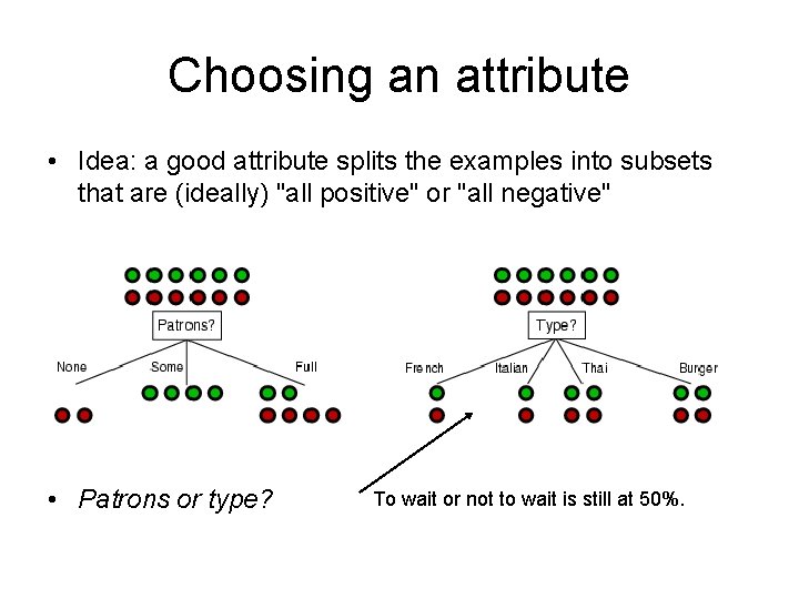
Choosing an attribute • Idea: a good attribute splits the examples into subsets that are (ideally) "all positive" or "all negative" • Patrons or type? To wait or not to wait is still at 50%.

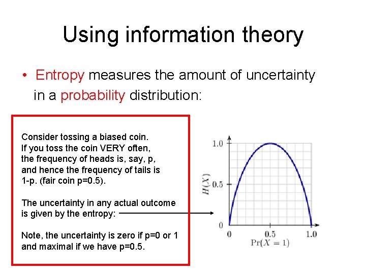
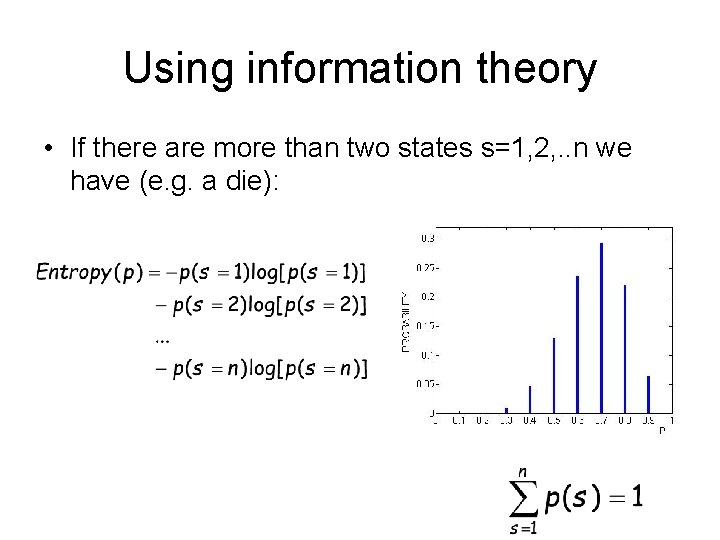
Using information theory • Entropy measures the amount of uncertainty in a probability distribution: Consider tossing a biased coin. If you toss the coin VERY often, the frequency of heads is, say, p, and hence the frequency of tails is 1 -p. (fair coin p=0. 5). The uncertainty in any actual outcome is given by the entropy: Note, the uncertainty is zero if p=0 or 1 and maximal if we have p=0. 5.

Using information theory • If there are more than two states s=1, 2, . . n we have (e. g. a die):

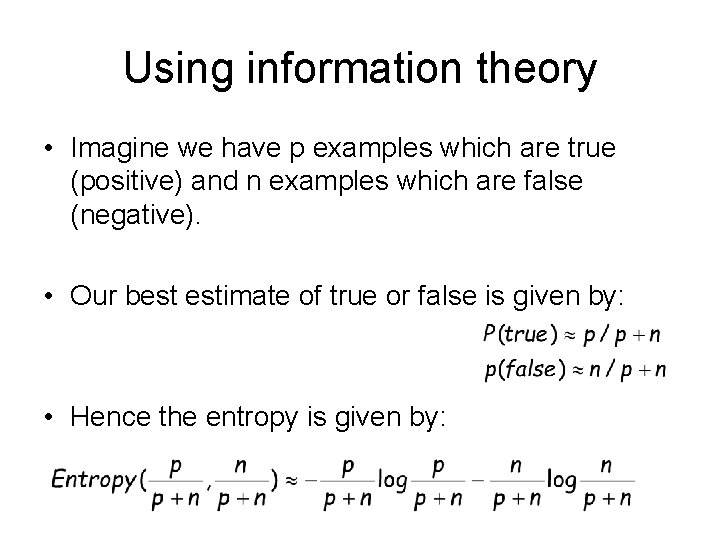
Using information theory • Imagine we have p examples which are true (positive) and n examples which are false (negative). • Our best estimate of true or false is given by: • Hence the entropy is given by:

Using Information Theory • How much information do we gain if we disclose the value of some attribute? • Answer: uncertainty before minus uncertainty after

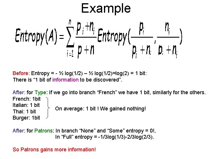
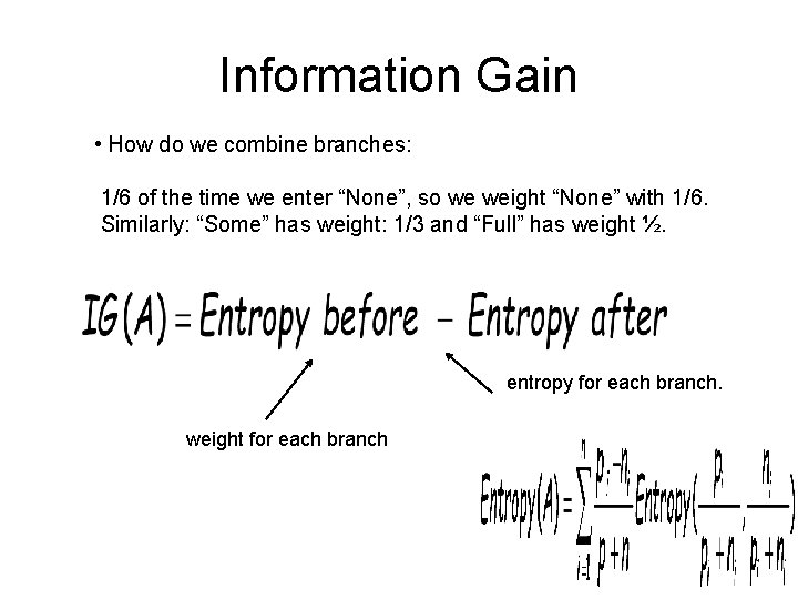
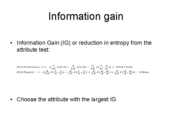
Example Before: Entropy = - ½ log(1/2) – ½ log(1/2)=log(2) = 1 bit: There is “ 1 bit of information to be discovered”. After: for Type: If we go into branch “French” we have 1 bit, similarly for the others. French: 1 bit Italian: 1 bit On average: 1 bit ! We gained nothing! Thai: 1 bit Burger: 1 bit After: for Patrons: In branch “None” and “Some” entropy = 0!, In “Full” entropy = -1/3 log(1/3)-2/3 log(2/3). So Patrons gains more information!

Information Gain • How do we combine branches: 1/6 of the time we enter “None”, so we weight “None” with 1/6. Similarly: “Some” has weight: 1/3 and “Full” has weight ½. entropy for each branch. weight for each branch

Information gain • Information Gain (IG) or reduction in entropy from the attribute test: • Choose the attribute with the largest IG

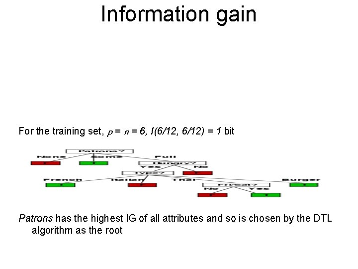
Information gain For the training set, p = n = 6, I(6/12, 6/12) = 1 bit Patrons has the highest IG of all attributes and so is chosen by the DTL algorithm as the root

Example contd. • Decision tree learned from the 12 examples: • Substantially simpler than “true” tree---a more complex hypothesis isn’t justified by small amount of data

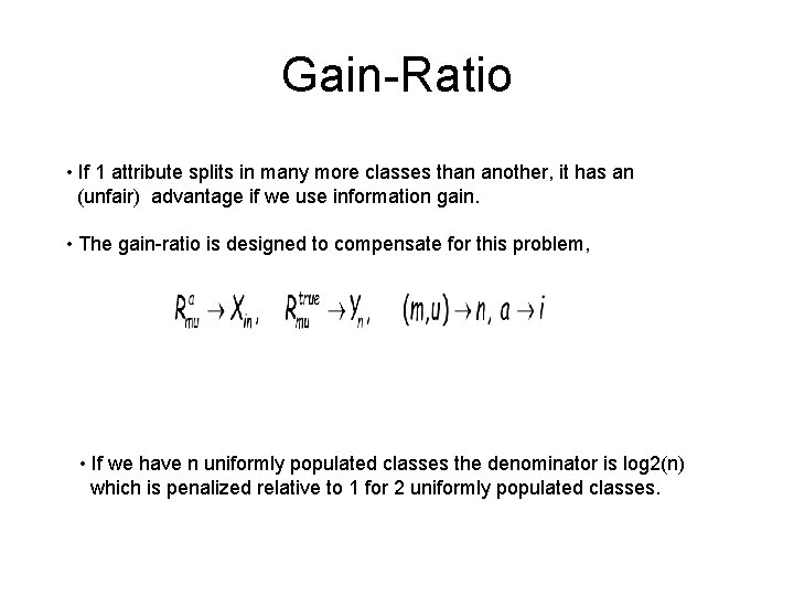
Gain-Ratio • If 1 attribute splits in many more classes than another, it has an (unfair) advantage if we use information gain. • The gain-ratio is designed to compensate for this problem, • If we have n uniformly populated classes the denominator is log 2(n) which is penalized relative to 1 for 2 uniformly populated classes.

What to Do if. . . • In some leaf there are no examples: Choose True or False according to the number of positive/negative examples at your parent. • There are no attributes left Two or more examples have the same attributes but different label: we have an error/noise. Stop and use majority vote. Demo: http: //www. cs. ubc. ca/labs/lci/CIspace/Version 4/d. Tree/

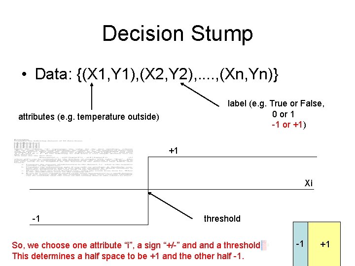
Continuous Variables • If variables are continuous we can bin them, or. . • We can learn a simple classifier on a single dimension • E. g. we can find decision point which classifies all data to the left of that point in one class and all data to the right in the other (decision stump – next slide) • We can also use a small subset of dimensions and train a linear classifier (e. g. logistic regression classifier).

Decision Stump • Data: {(X 1, Y 1), (X 2, Y 2), . . , (Xn, Yn)} label (e. g. True or False, 0 or 1 -1 or +1) attributes (e. g. temperature outside) +1 Xi -1 threshold So, we choose one attribute “i”, a sign “+/-” and a threshold This determines a half space to be +1 and the other half -1. -1 -1 +1

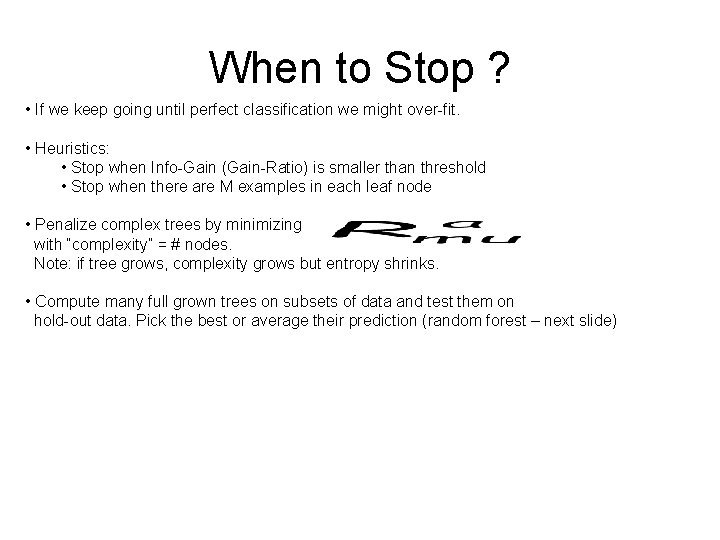
When to Stop ? • If we keep going until perfect classification we might over-fit. • Heuristics: • Stop when Info-Gain (Gain-Ratio) is smaller than threshold • Stop when there are M examples in each leaf node • Penalize complex trees by minimizing with “complexity” = # nodes. Note: if tree grows, complexity grows but entropy shrinks. • Compute many full grown trees on subsets of data and test them on hold-out data. Pick the best or average their prediction (random forest – next slide)

Pruning & Random Forests • Sometimes it is better to grow the trees all the way down and prune them back later. Later splits may become beneficial, but we wouldn’t see them if we stopped early. • We simply consider all leaf nodes and consider them for elimination, using any of the above criteria. • Alternatively, we grow many trees on datasets sampled from the original dataset with replacement (a bootstrap sample). • Draw K bootstrap samples of size N • Grow a DT, randomly sampling one or a few attributes/dimensions to split on • Average the predictions of the trees for a new query (or take majority vote) • Evaluation: for each bootstrap sample about 30% of the data was left out. For each data-item determine which trees did not use that data-case and test performance using this sub-ensemble of trees. This is a conservative estimate, because in reality there are more trees. • Random Forests are state of the art classifiers!

Bagging • The idea behind random forests can be applied to any classifier and is called bagging: • Sample M bootstrap samples. • Train M different classifiers on these bootstrap samples • For a new query, let all classifiers predict and take an average (or majority vote) • The basic idea that this works is that if the classifiers make independent errors, then their ensemble can improve performance.

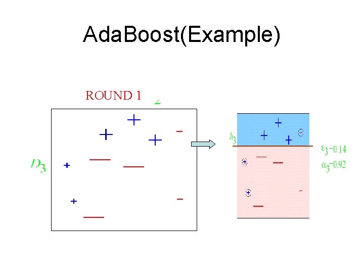
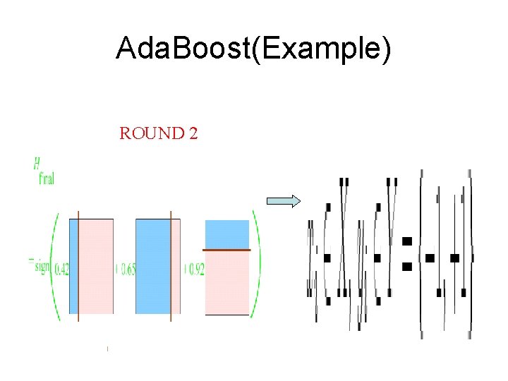
Boosting • Main idea: – train classifiers (e. g. decision trees) in a sequence. – a new classifier should focus on those cases which were incorrectly classified in the last round. – combine the classifiers by letting them vote on the final prediction (like bagging). – each classifier could be (should be) very “weak”, e. g. a decision stump.

Example this line is one simple classifier saying that everything to the left + and everything to the right is -

Boosting Intuition • We adaptively weigh each data case. • Data cases which are wrongly classified get high weight (the algorithm will focus on them) • Each boosting round learns a new (simple) classifier on the weighed dataset. • These classifiers are weighed to combine them into a single powerful classifier. • Classifiers that obtain low training error rate have high weight. • We stop by using monitoring a hold out set (cross-validation).

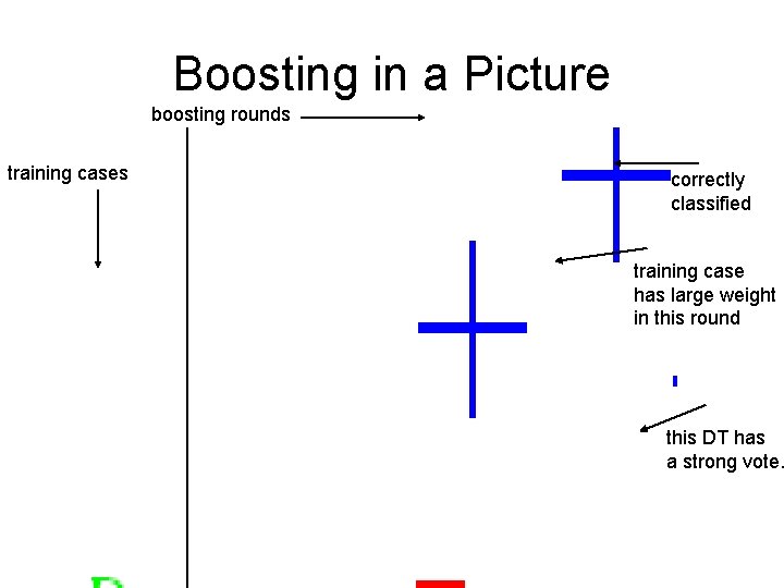
Boosting in a Picture boosting rounds training cases correctly classified training case has large weight in this round this DT has a strong vote.

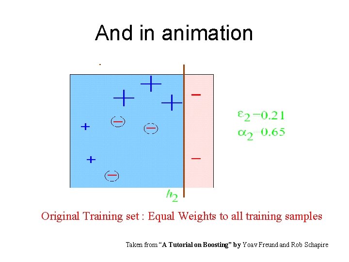
And in animation Original Training set : Equal Weights to all training samples Taken from “A Tutorial on Boosting” by Yoav Freund and Rob Schapire

Ada. Boost(Example) ROUND 1

Ada. Boost(Example) ROUND 2

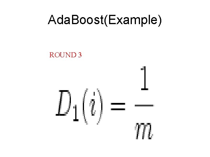
Ada. Boost(Example) ROUND 3

Ada. Boost(Example)

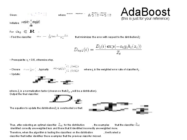
Given: where Ada. Boost (this is just for your reference) Initialise . For : • Find the classifier that minimizes the error with respect to the distribution Dt: • Prerequisite: εt < 0. 5, otherwise stop. • Choose , typically where εt is the weighted error rate of classifier ht. • Update: where Zt is a normalisation factor (chosen so that Dt + 1 will be a distribution). Output the final classifier: The equation to update the distribution Dt is constructed so that: Thus, after selecting an optimal classifier for the distribution , the examples that the classifier identified correctly are weighted less and those that it identified incorrectly are weighted more. Therefore, when the algorithm is testing the classifiers on the distribution , it will select a classifier that better identifies those examples that the previous classifer missed.

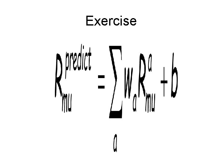
Exercise

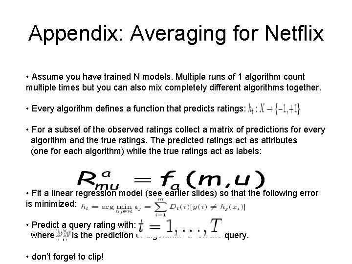
Appendix: Averaging for Netflix • Assume you have trained N models. Multiple runs of 1 algorithm count multiple times but you can also mix completely different algorithms together. • Every algorithm defines a function that predicts ratings: • For a subset of the observed ratings collect a matrix of predictions for every algorithm and the true ratings. The predicted ratings act as attributes (one for each algorithm) while the true ratings act as labels: • Fit a linear regression model (see earlier slides) so that the following error is minimized: • Predict a query rating with: where is the prediction of algorithm “a” on the query. • don’t forget to clip!