STT 592 002 Intro to Statistical Learning 1

STT 592 -002: Intro. to Statistical Learning 1 UNSUPERVISED LEARNING Chapter 10 Disclaimer: This PPT is modified based on IOM 530: Intro. to Statistical Learning

STT 592 -002: Intro. to Statistical Learning WHAT IS CLUSTERING? 2

STT 592 -002: Intro. to Statistical Learning 3 PCA and Clustering • PCA looks to find a low-dimensional representation of the observations that explain a good fraction of the variance; • Clustering looks to find homogeneous subgroups among the observations.

STT 592 -002: Intro. to Statistical Learning 4 Review: Examples of Unsupervised Learning • Eg: A cancer researcher might assay gene expression levels in 100 patients with breast cancer, and look for subgroups among the breast cancer samples, or among the genes, in order to obtain a better understanding of the disease. • Eg: Online shopping site: identify groups of shoppers with similar browsing and purchase histories, as well as items of interest within each group. Then an individual shopper can be preferentially shown the items likely to be interested, based on the purchase histories of similar shoppers. A search engine choose search results to display to a particular individual based on the click histories of other individuals with similar search patterns.

STT 592 -002: Intro. to Statistical Learning 5 Clustering • Clustering refers to a set of techniques for finding subgroups, or clusters, in a data set. • A good clustering is one when the observations within a group are similar but between groups are very different • For example, suppose we collect p measurements on each of n breast cancer patients. There may be different unknown types of cancer which we could discover by clustering the data

STT 592 -002: Intro. to Statistical Learning 6 Different Clustering Methods • There are many different types of clustering methods • We will concentrate on two of the most commonly used approaches: • K-Means Clustering • Hierarchical Clustering

STT 592 -002: Intro. to Statistical Learning K-MEANS CLUSTERING 7

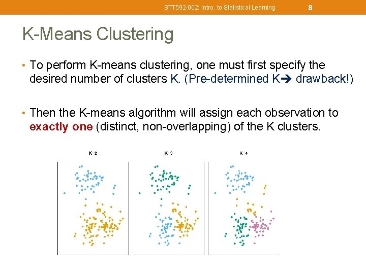
STT 592 -002: Intro. to Statistical Learning 8 K-Means Clustering • To perform K-means clustering, one must first specify the desired number of clusters K. (Pre-determined K drawback!) • Then the K-means algorithm will assign each observation to exactly one (distinct, non-overlapping) of the K clusters.

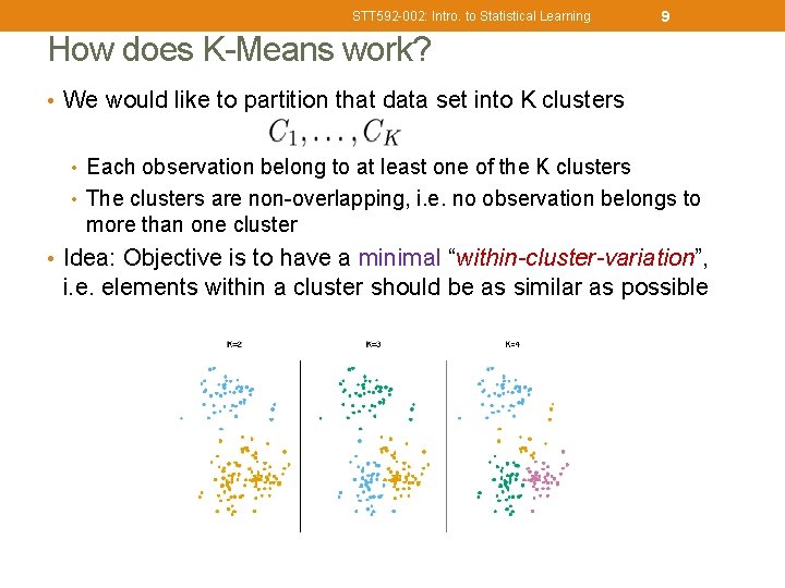
STT 592 -002: Intro. to Statistical Learning 9 How does K-Means work? • We would like to partition that data set into K clusters • Each observation belong to at least one of the K clusters • The clusters are non-overlapping, i. e. no observation belongs to more than one cluster • Idea: Objective is to have a minimal “within-cluster-variation”, i. e. elements within a cluster should be as similar as possible

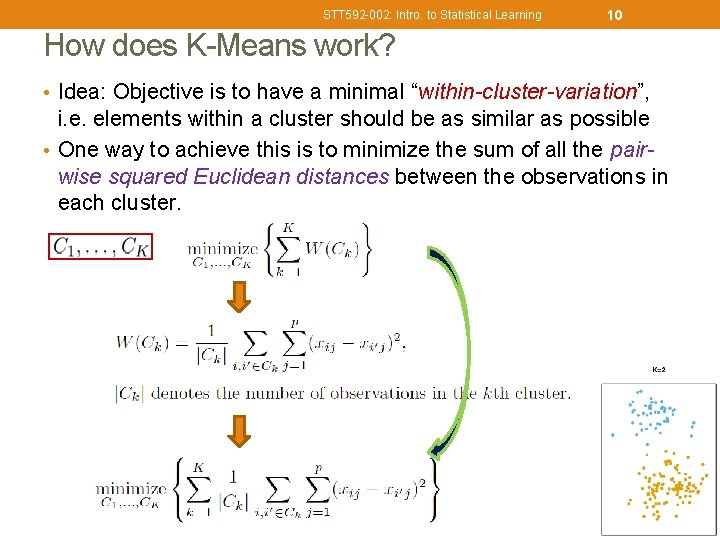
STT 592 -002: Intro. to Statistical Learning 10 How does K-Means work? • Idea: Objective is to have a minimal “within-cluster-variation”, i. e. elements within a cluster should be as similar as possible • One way to achieve this is to minimize the sum of all the pairwise squared Euclidean distances between the observations in each cluster.

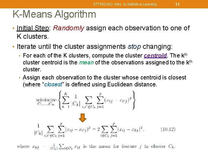
STT 592 -002: Intro. to Statistical Learning 11 K-Means Algorithm • Initial Step: Randomly assign each observation to one of K clusters. • Iterate until the cluster assignments stop changing: • For each of the K clusters, compute the cluster centroid. The kth cluster centroid is the mean of the observations assigned to the kth cluster. • Assign each observation to the cluster whose centroid is closest (where “closest” is defined using Euclidean distance.

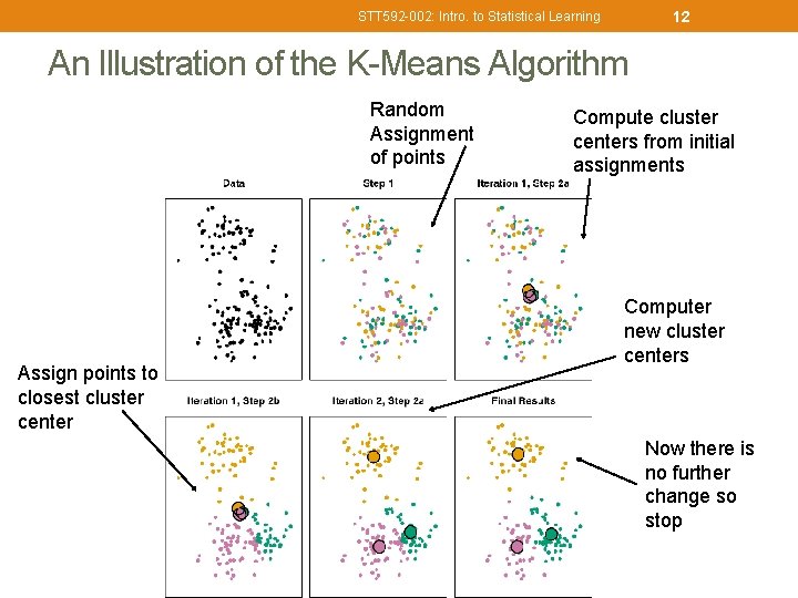
12 STT 592 -002: Intro. to Statistical Learning An Illustration of the K-Means Algorithm Random Assignment of points Assign points to closest cluster center Compute cluster centers from initial assignments Computer new cluster centers Now there is no further change so stop

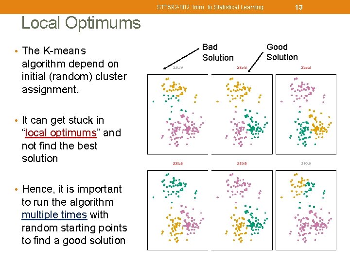
STT 592 -002: Intro. to Statistical Learning 13 Local Optimums • The K-means algorithm depend on initial (random) cluster assignment. • It can get stuck in “local optimums” and not find the best solution • Hence, it is important to run the algorithm multiple times with random starting points to find a good solution Bad Solution Good Solution

STT 592 -002: Intro. to Statistical Learning HIERARCHICAL CLUSTERING 14

STT 592 -002: Intro. to Statistical Learning 15 Hierarchical Clustering • K-Means clustering requires choosing the number of clusters K. • If we don’t want to do that, an alternative is to use Hierarchical Clustering • Hierarchical Clustering has an added advantage that it produces a tree based representation of the observations, called a Dendrogram • Bottom-up, or agglomerative clustering will be covered.

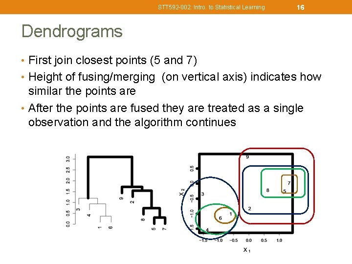
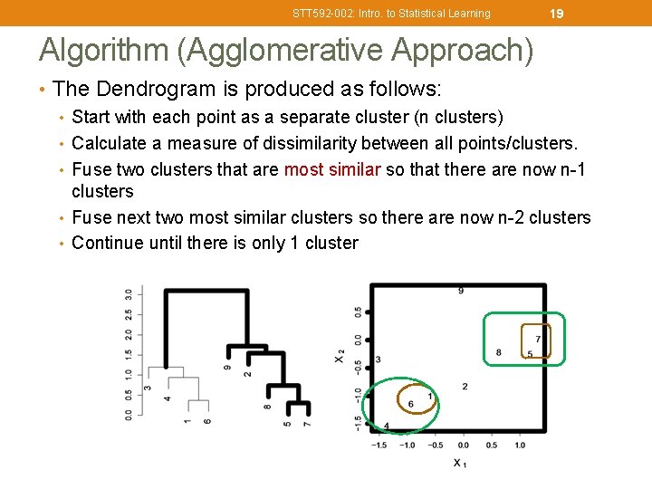
STT 592 -002: Intro. to Statistical Learning 16 Dendrograms • First join closest points (5 and 7) • Height of fusing/merging (on vertical axis) indicates how similar the points are • After the points are fused they are treated as a single observation and the algorithm continues

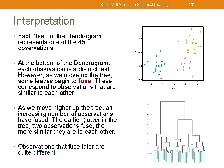
STT 592 -002: Intro. to Statistical Learning Interpretation • Each “leaf” of the Dendrogram represents one of the 45 observations • At the bottom of the Dendrogram, each observation is a distinct leaf. However, as we move up the tree, some leaves begin to fuse. These correspond to observations that are similar to each other. • As we move higher up the tree, an increasing number of observations have fused. The earlier (lower in the tree) two observations fuse, the more similar they are to each other. • Observations that fuse later are quite different 17

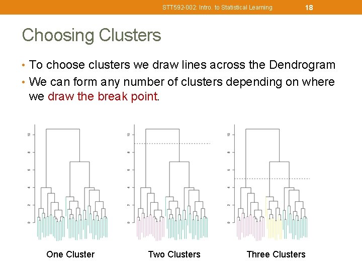
STT 592 -002: Intro. to Statistical Learning 18 Choosing Clusters • To choose clusters we draw lines across the Dendrogram • We can form any number of clusters depending on where we draw the break point. One Cluster Two Clusters Three Clusters

STT 592 -002: Intro. to Statistical Learning 19 Algorithm (Agglomerative Approach) • The Dendrogram is produced as follows: • Start with each point as a separate cluster (n clusters) • Calculate a measure of dissimilarity between all points/clusters. • Fuse two clusters that are most similar so that there are now n-1 clusters • Fuse next two most similar clusters so there are now n-2 clusters • Continue until there is only 1 cluster

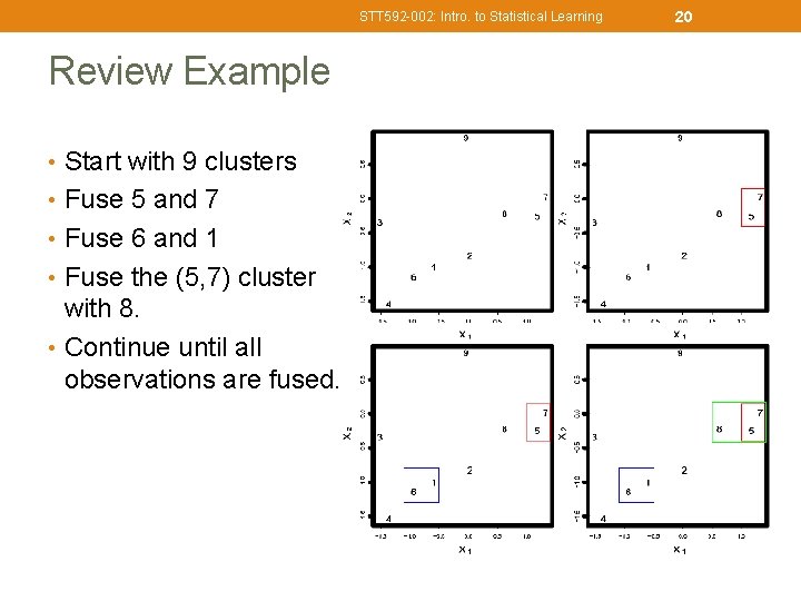
STT 592 -002: Intro. to Statistical Learning Review Example • Start with 9 clusters • Fuse 5 and 7 • Fuse 6 and 1 • Fuse the (5, 7) cluster with 8. • Continue until all observations are fused. 20

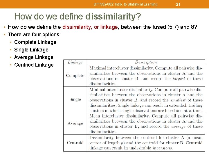
STT 592 -002: Intro. to Statistical Learning 21 How do we define dissimilarity? • How do we define the dissimilarity, or linkage, between the fused (5, 7) and 8? • There are four options: • Complete Linkage • Single Linkage • Average Linkage • Centriod Linkage

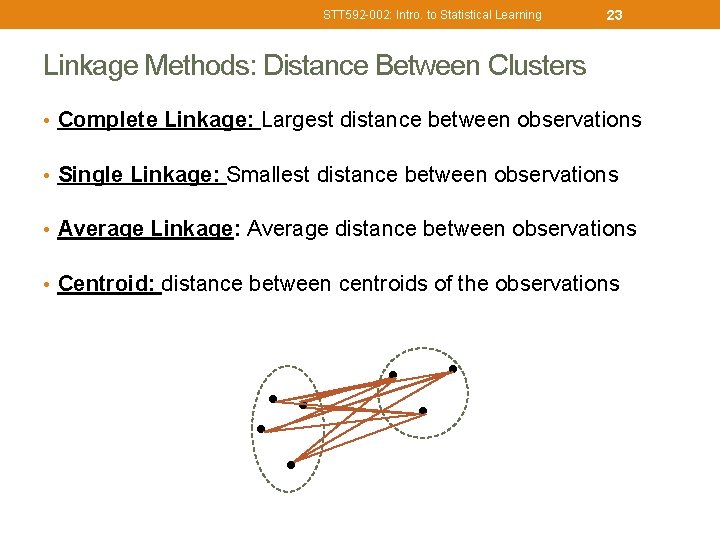
STT 592 -002: Intro. to Statistical Learning 22 Linkage Methods: Distance Between Clusters • Complete Linkage: Largest distance between observations • Single Linkage: Smallest distance between observations • Average Linkage: Average distance between observations • Centroid: distance between centroids of the observations

STT 592 -002: Intro. to Statistical Learning 23 Linkage Methods: Distance Between Clusters • Complete Linkage: Largest distance between observations • Single Linkage: Smallest distance between observations • Average Linkage: Average distance between observations • Centroid: distance between centroids of the observations

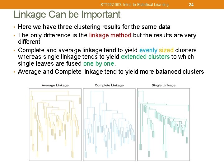
STT 592 -002: Intro. to Statistical Learning 24 Linkage Can be Important • Here we have three clustering results for the same data • The only difference is the linkage method but the results are very different • Complete and average linkage tend to yield evenly sized clusters whereas single linkage tends to yield extended clusters to which single leaves are fused one by one. • Average and Complete linkage tend to yield more balanced clusters.

STT 592 -002: Intro. to Statistical Learning 25 Choice of Dissimilarity Measure • So far, we have considered using Euclidean distance as the dissimilarity measure • However, an alternative measure that could make sense in some cases is the correlation based distance

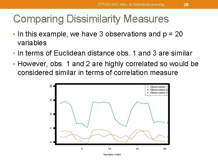
STT 592 -002: Intro. to Statistical Learning 26 Comparing Dissimilarity Measures • In this example, we have 3 observations and p = 20 variables • In terms of Euclidean distance obs. 1 and 3 are similar • However, obs. 1 and 2 are highly correlated so would be considered similar in terms of correlation measure

STT 592 -002: Intro. to Statistical Learning 27 Online Shopping Example • Suppose we record the number of purchases of each item (columns) for each customer (rows) • Using Euclidean distance, customers who have purchased very little will be clustered together • Using correlation measure, customers who tend to purchase the same types of products will be clustered together even if the magnitude of their purchase may be quite different

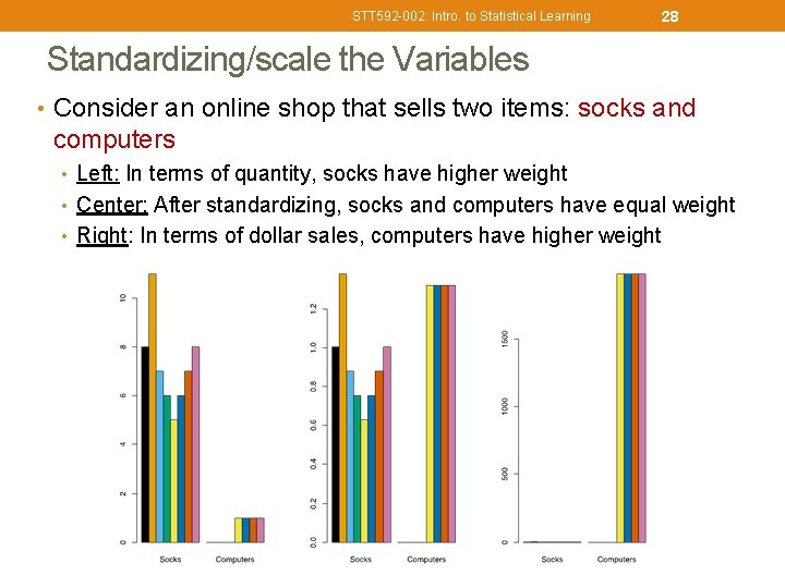
STT 592 -002: Intro. to Statistical Learning 28 Standardizing/scale the Variables • Consider an online shop that sells two items: socks and computers • Left: In terms of quantity, socks have higher weight • Center: After standardizing, socks and computers have equal weight • Right: In terms of dollar sales, computers have higher weight

STT 592 -002: Intro. to Statistical Learning FINAL THOUGHTS 29

STT 592 -002: Intro. to Statistical Learning 30 Practical Issues in Clustering • In order to perform clustering, some decisions must be made: • Should the features first be standardized? i. e. Have the variables centered to have a mean of zero and standard deviation of one. • In case of hierarchical clustering: • What dissimilarity measure should be used? • What type of linkage should be used? • Where should we cut the Dendrogram in order to obtain clusters? • In case of K-means clustering: • How many clusters K should we look for the data? • In practice, we try several different choices, and look for the one with the most useful or interpretable solution. There is no single right answer!

STT 592 -002: Intro. to Statistical Learning 31 Final Thoughts • Most importantly, one must be careful about how the results of a clustering analysis are reported • These results should NOT be taken as the absolute truth about a data set • Rather, they should constitute a starting point for the developments of a scientific hypothesis and further study, preferably on independent data Exploratory data analysis