STT 592 002 Intro to Statistical Learning SUPPORT

STT 592 -002: Intro. to Statistical Learning SUPPORT VECTOR MACHINES (SVM) Chapter 09 Disclaimer: This PPT is modified based on IOM 530: Intro. to Statistical Learning 1

9. 1 SUPPORT VECTOR CLASSIFIER

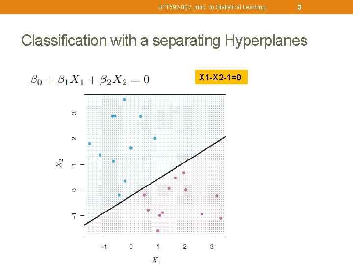
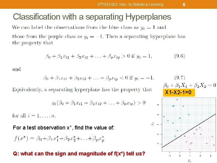
STT 592 -002: Intro. to Statistical Learning 3 Classification with a separating Hyperplanes X 1 -X 2 -1=0

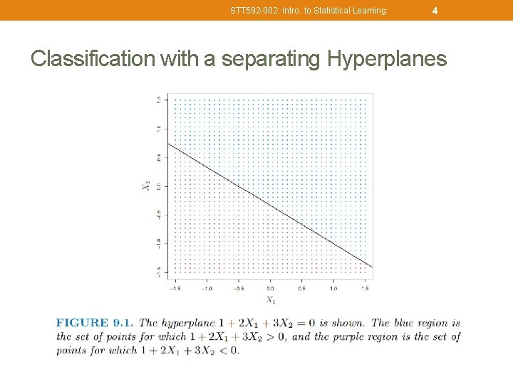
STT 592 -002: Intro. to Statistical Learning 4 Classification with a separating Hyperplanes

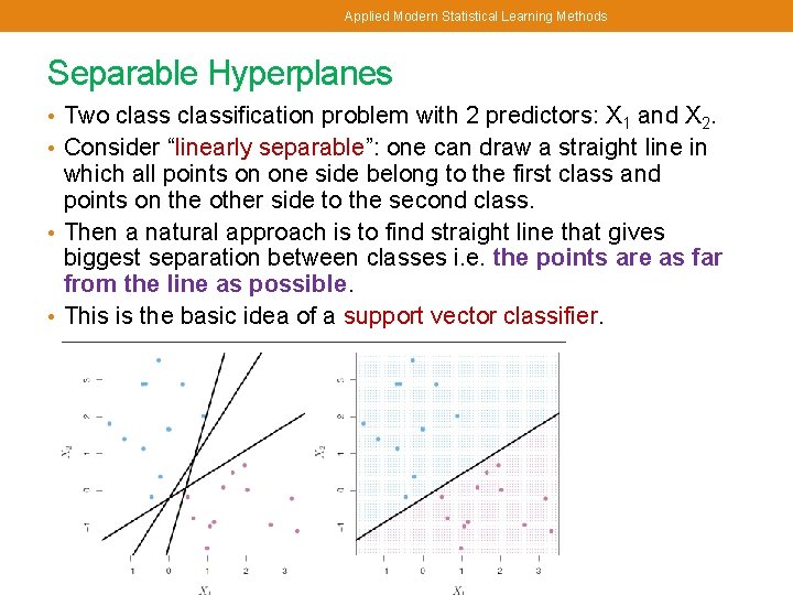
Applied Modern Statistical Learning Methods Separable Hyperplanes • Two classification problem with 2 predictors: X 1 and X 2. • Consider “linearly separable”: one can draw a straight line in which all points on one side belong to the first class and points on the other side to the second class. • Then a natural approach is to find straight line that gives biggest separation between classes i. e. the points are as far from the line as possible. • This is the basic idea of a support vector classifier.

6 STT 592 -002: Intro. to Statistical Learning Classification with a separating Hyperplanes X 1 -X 2 -1=0 For a test observation x*, find the value of: Q: what can the sign and magnitude of f(x*) tell us?

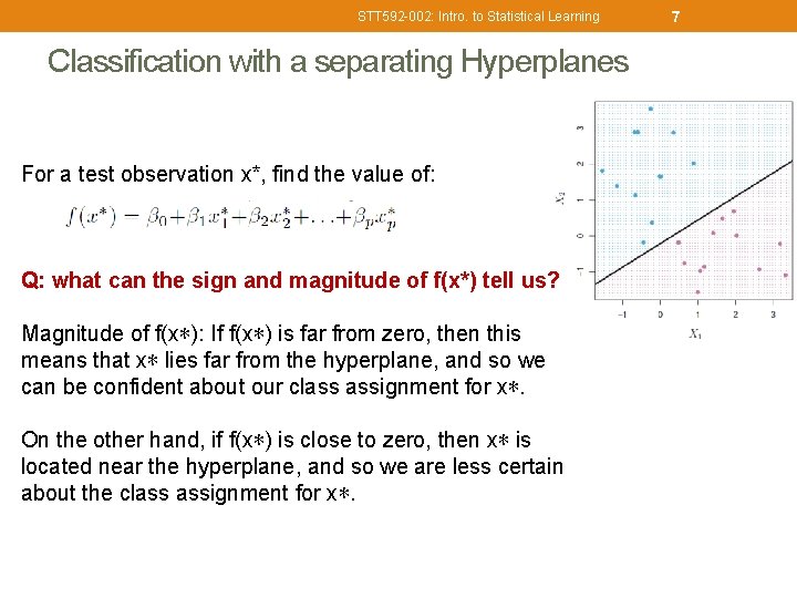
STT 592 -002: Intro. to Statistical Learning Classification with a separating Hyperplanes For a test observation x*, find the value of: Q: what can the sign and magnitude of f(x*) tell us? Magnitude of f(x∗): If f(x∗) is far from zero, then this means that x∗ lies far from the hyperplane, and so we can be confident about our class assignment for x∗. On the other hand, if f(x∗) is close to zero, then x∗ is located near the hyperplane, and so we are less certain about the class assignment for x∗. 7

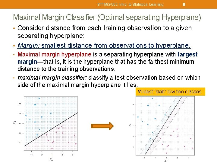
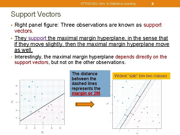
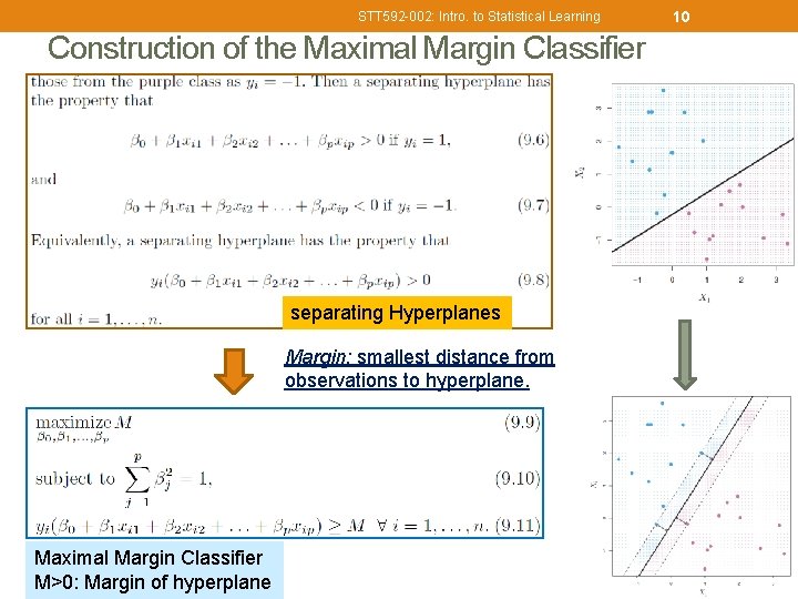
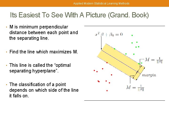
STT 592 -002: Intro. to Statistical Learning 8 Maximal Margin Classifier (Optimal separating Hyperplane) • Consider distance from each training observation to a given separating hyperplane; • Margin: smallest distance from observations to hyperplane. • Maximal margin hyperplane is a separating hyperplane with largest margin—that is, it is the hyperplane that has the farthest minimum distance to the training observations. • maximal margin classifier: classify a test observation based on which side of the maximal margin hyperplane it lies. Widest “slab” b/w two classes

STT 592 -002: Intro. to Statistical Learning 9 Support Vectors • Right panel figure: Three observations are known as support vectors. • They support the maximal margin hyperplane, in the sense that if they move slightly, then the maximal margin hyperplane move as well. • Interestingly, the maximal margin hyperplane depends directly on the support vectors, but not on the other observations. The distance between the dashed lines represents the margin or 2 M. Widest “slab” b/w two classes

STT 592 -002: Intro. to Statistical Learning Construction of the Maximal Margin Classifier separating Hyperplanes Margin: smallest distance from observations to hyperplane. Maximal Margin Classifier M>0: Margin of hyperplane 10

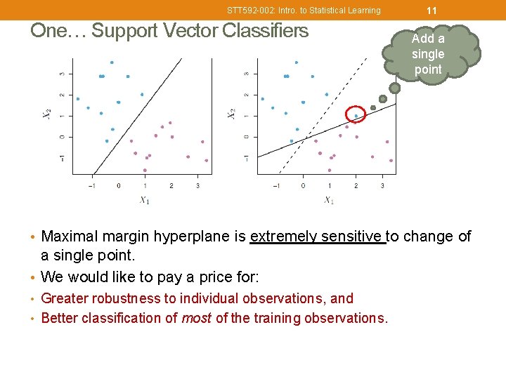
STT 592 -002: Intro. to Statistical Learning One… Support Vector Classifiers 11 Add a single point • Maximal margin hyperplane is extremely sensitive to change of a single point. • We would like to pay a price for: • Greater robustness to individual observations, and • Better classification of most of the training observations.

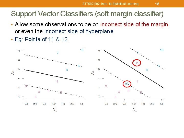
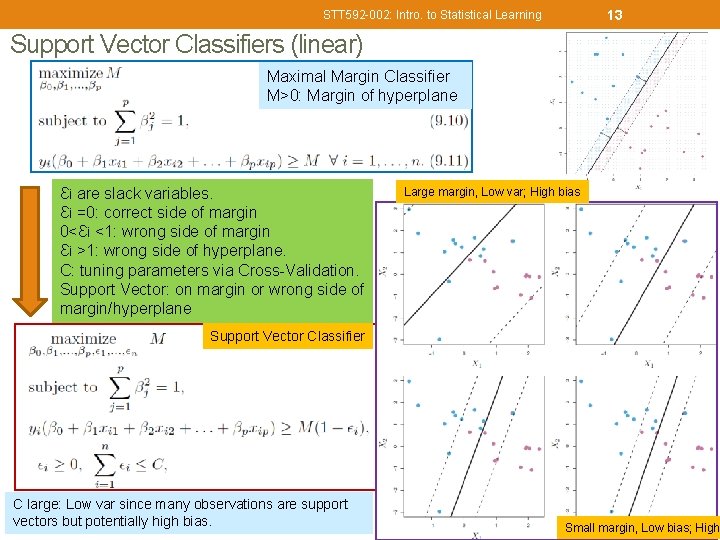
STT 592 -002: Intro. to Statistical Learning 12 Support Vector Classifiers (soft margin classifier) • Allow some observations to be on incorrect side of the margin, or even the incorrect side of hyperplane • Eg: Points of 11 & 12.

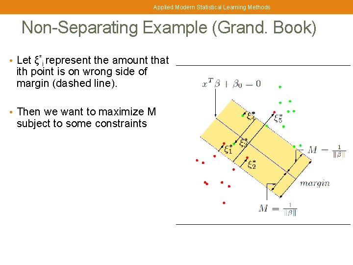
13 STT 592 -002: Intro. to Statistical Learning Support Vector Classifiers (linear) Maximal Margin Classifier M>0: Margin of hyperplane Ɛi are slack variables. Ɛi =0: correct side of margin 0<Ɛi <1: wrong side of margin Ɛi >1: wrong side of hyperplane. C: tuning parameters via Cross-Validation. Support Vector: on margin or wrong side of margin/hyperplane Large margin, Low var; High bias Support Vector Classifier C large: Low var since many observations are support vectors but potentially high bias. Small margin, Low bias; High

Applied Modern Statistical Learning Methods Its Easiest To See With A Picture (Grand. Book) • M is minimum perpendicular distance between each point and the separating line. • Find the line which maximizes M. • This line is called the “optimal separating hyperplane”. • The classification of a point depends on which side of the line it falls on.

Applied Modern Statistical Learning Methods Non-Separating Example (Grand. Book) • Let ξ*i represent the amount that ith point is on wrong side of margin (dashed line). • Then we want to maximize M subject to some constraints

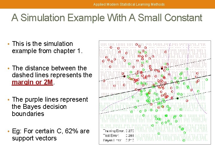
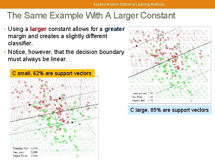
Applied Modern Statistical Learning Methods A Simulation Example With A Small Constant • This is the simulation example from chapter 1. • The distance between the dashed lines represents the margin or 2 M. • The purple lines represent the Bayes decision boundaries • Eg: For certain C, 62% are support vectors

Applied Modern Statistical Learning Methods The Same Example With A Larger Constant • Using a larger constant allows for a greater margin and creates a slightly different classifier. • Notice, however, that the decision boundary must always be linear. C small, 62% are support vectors C large, 85% are support vectors

9. 2 SUPPORT VECTOR MACHINE CLASSIFIER

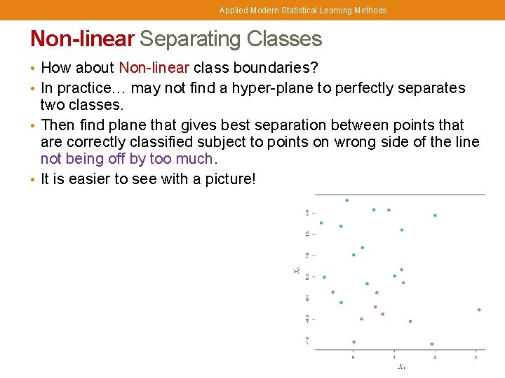
Applied Modern Statistical Learning Methods Non-linear Separating Classes • How about Non-linear class boundaries? • In practice… may not find a hyper-plane to perfectly separates two classes. • Then find plane that gives best separation between points that are correctly classified subject to points on wrong side of the line not being off by too much. • It is easier to see with a picture!

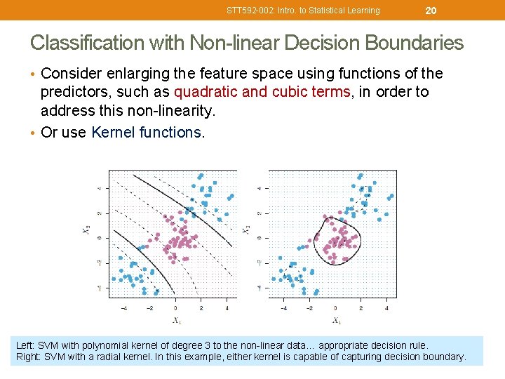
STT 592 -002: Intro. to Statistical Learning 20 Classification with Non-linear Decision Boundaries • Consider enlarging the feature space using functions of the predictors, such as quadratic and cubic terms, in order to address this non-linearity. • Or use Kernel functions. Left: SVM with polynomial kernel of degree 3 to the non-linear data… appropriate decision rule. Right: SVM with a radial kernel. In this example, either kernel is capable of capturing decision boundary.

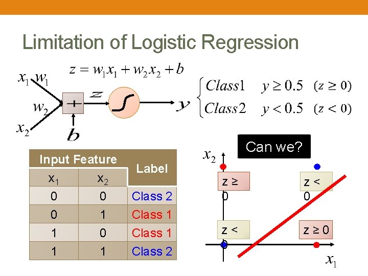
Limitation of Logistic Regression Input Feature x 1 x 2 0 0 0 1 1 1 0 1 Can we? Label Class 2 Class 1 Class 2 z ≥ 0 z < 0 z ≥ 0

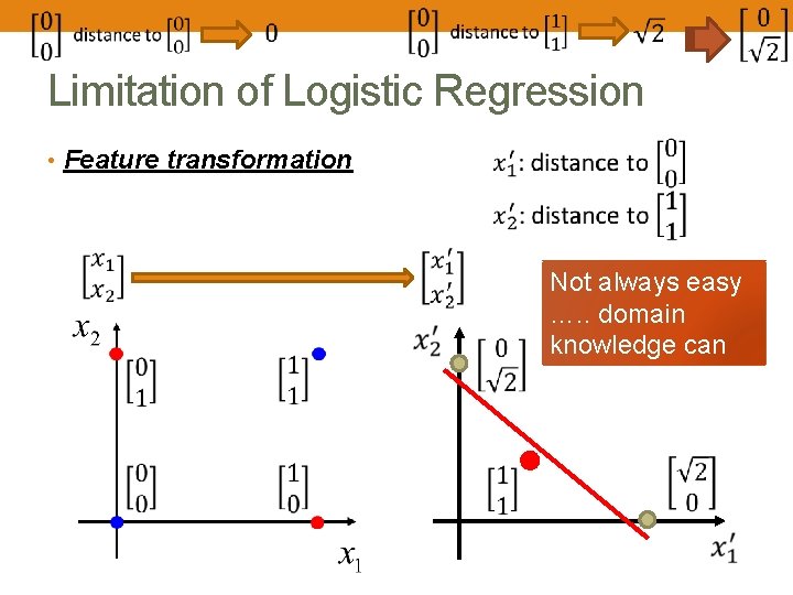
Limitation of Logistic Regression • Feature transformation Not always easy …. . domain knowledge can be helpful

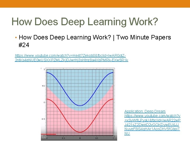
How Does Deep Learning Work? • How Does Deep Learning Work? | Two Minute Papers #24 https: //www. youtube. com/watch? v=He 4 t 7 Zekob 0&fbclid=Iw. AR 0 ot. Z 2 nt. Ks 4 e. NUE 0 w. USXXPZMLZKj. DJwr. Hj 3 s. Htnz 8 a 4 Xb. PMRk-EXw 5 R 1 k Application: Deep Dream https: //www. youtube. com/watch? v =x. Sy. Wfi. LPya. U&fbclid=Iw. AR 22 w. P J 421 s. Z 2 Dwe. D 2 v. GOKDyw. EU 6 JJ Nuye. F 8 i. S 4 g. HAr 1 Aos. Dh. V 5 f. Gbpi. T NU

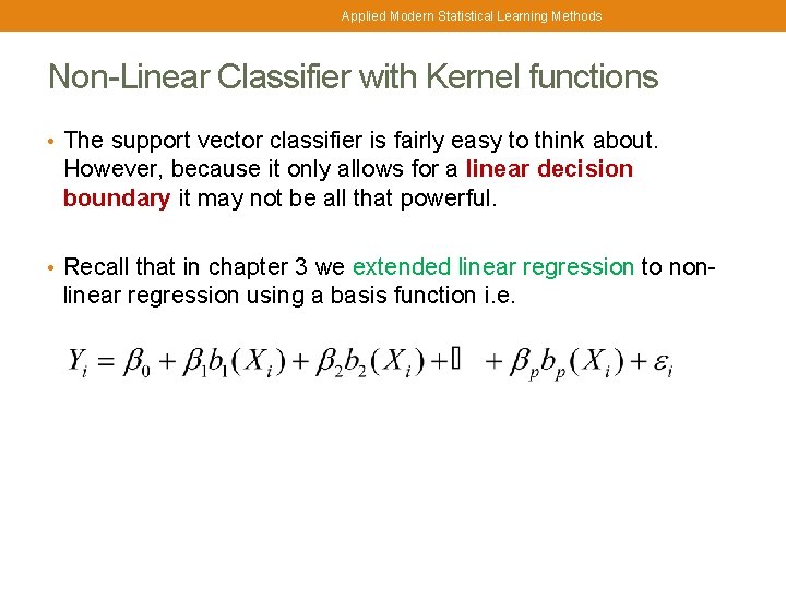
Applied Modern Statistical Learning Methods Non-Linear Classifier with Kernel functions • The support vector classifier is fairly easy to think about. However, because it only allows for a linear decision boundary it may not be all that powerful. • Recall that in chapter 3 we extended linear regression to non- linear regression using a basis function i. e.

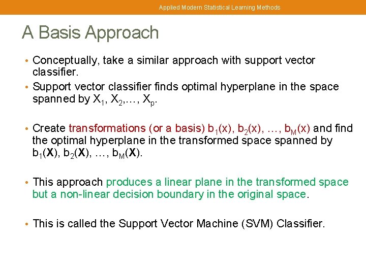
Applied Modern Statistical Learning Methods A Basis Approach • Conceptually, take a similar approach with support vector classifier. • Support vector classifier finds optimal hyperplane in the space spanned by X 1, X 2, …, Xp. • Create transformations (or a basis) b 1(x), b 2(x), …, b. M(x) and find the optimal hyperplane in the transformed space spanned by b 1(X), b 2(X), …, b. M(X). • This approach produces a linear plane in the transformed space but a non-linear decision boundary in the original space. • This is called the Support Vector Machine (SVM) Classifier.

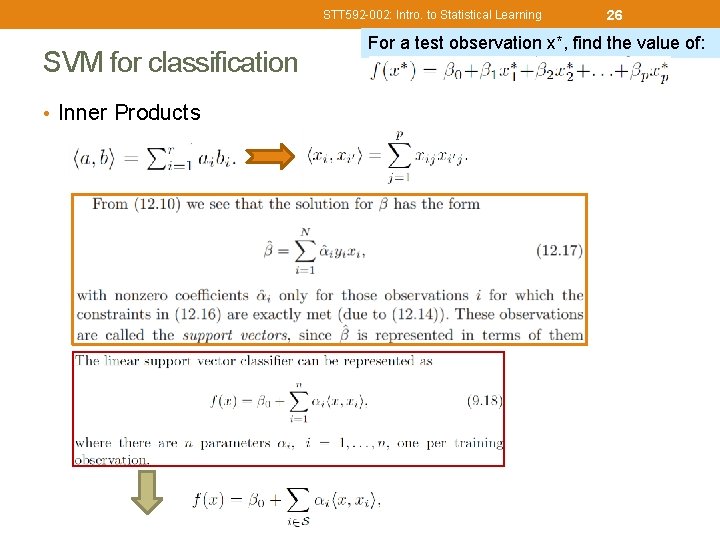
STT 592 -002: Intro. to Statistical Learning SVM for classification • Inner Products 26 For a test observation x*, find the value of:

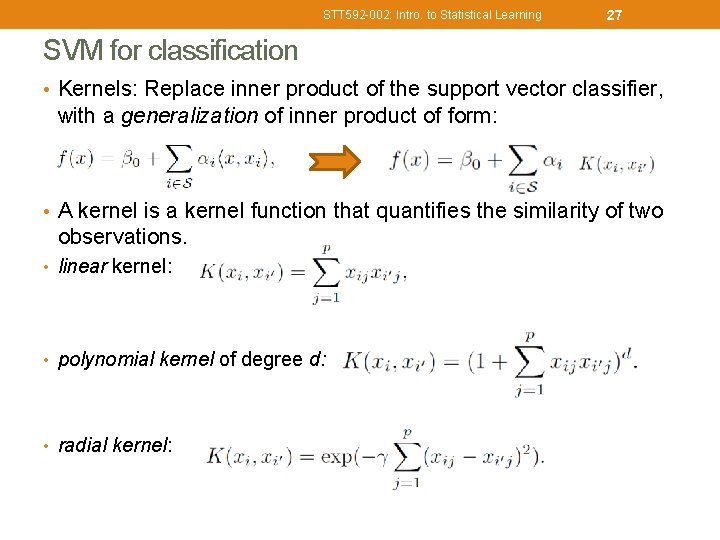
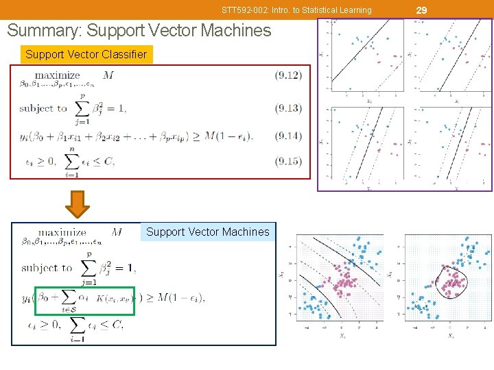
STT 592 -002: Intro. to Statistical Learning 27 SVM for classification • Kernels: Replace inner product of the support vector classifier, with a generalization of inner product of form: • A kernel is a kernel function that quantifies the similarity of two observations. • linear kernel: • polynomial kernel of degree d: • radial kernel:

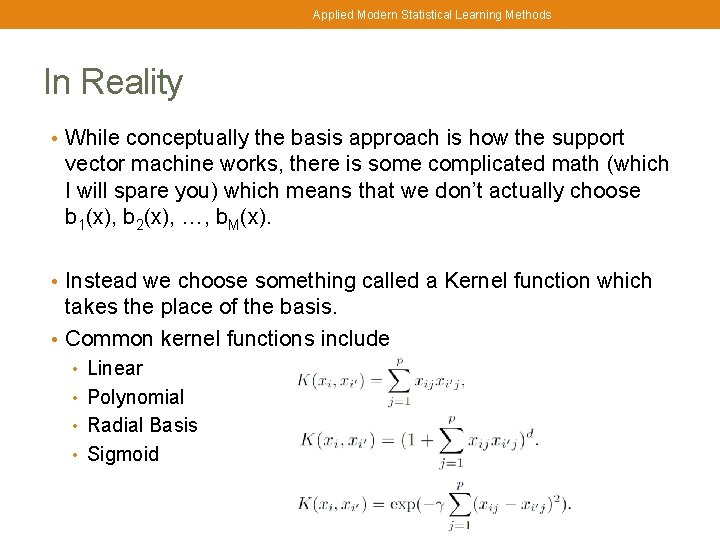
Applied Modern Statistical Learning Methods In Reality • While conceptually the basis approach is how the support vector machine works, there is some complicated math (which I will spare you) which means that we don’t actually choose b 1(x), b 2(x), …, b. M(x). • Instead we choose something called a Kernel function which takes the place of the basis. • Common kernel functions include • Linear • Polynomial • Radial Basis • Sigmoid

STT 592 -002: Intro. to Statistical Learning Summary: Support Vector Machines Support Vector Classifier Support Vector Machines 29

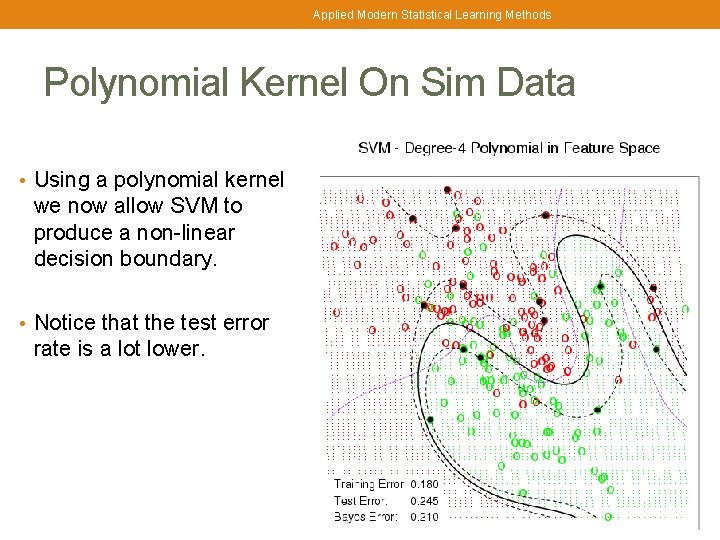
Applied Modern Statistical Learning Methods Polynomial Kernel On Sim Data • Using a polynomial kernel we now allow SVM to produce a non-linear decision boundary. • Notice that the test error rate is a lot lower.

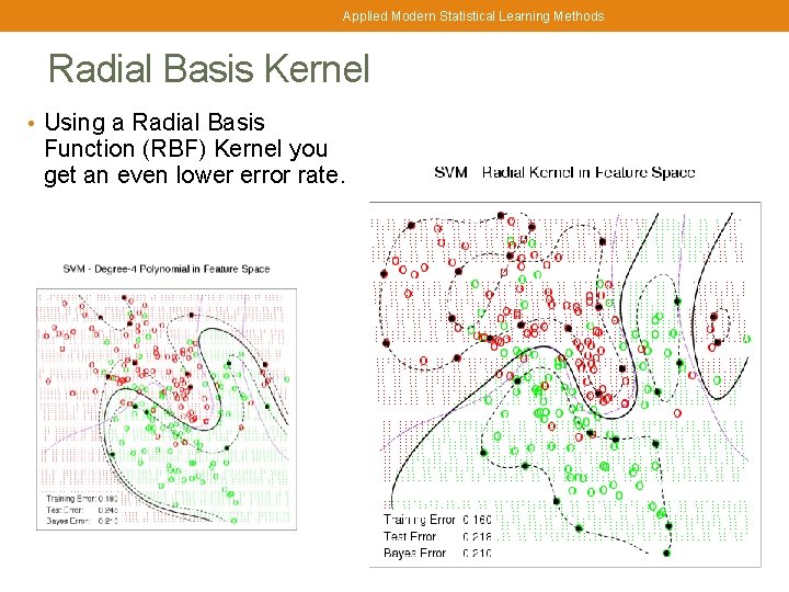
Applied Modern Statistical Learning Methods Radial Basis Kernel • Using a Radial Basis Function (RBF) Kernel you get an even lower error rate.

Applied Modern Statistical Learning Methods More Than Two Predictors • This idea works just as well with more than two predictors. • For example, with three predictors you want to find the plane that produces the largest separation between the classes. • With more than three dimensions it becomes hard to visualize a plane but it still exists. In general they are caller hyper-planes. • One versus One: compare each pairs • One versus All: one of K classes v. s. all remaining K-1 classes.

REVIEW: CHAP 4 CHAP 8: HOW TO DRAW ROC CURVE

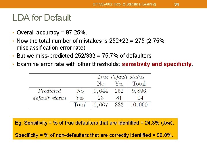
STT 592 -002: Intro. to Statistical Learning 34 LDA for Default • Overall accuracy = 97. 25%. • Now the total number of mistakes is 252+23 = 275 (2. 75% misclassification error rate) • But we miss-predicted 252/333 = 75. 7% of defaulters • Examine error rate with other thresholds: sensitivity and specificity. Eg: Sensitivity = % of true defaulters that are identified = 24. 3% (low). Specificity = % of non-defaulters that are correctly identified = 99. 8%.

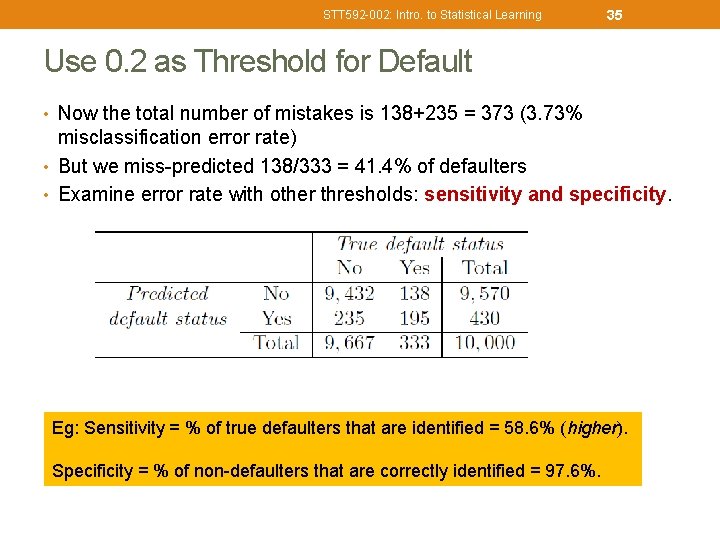
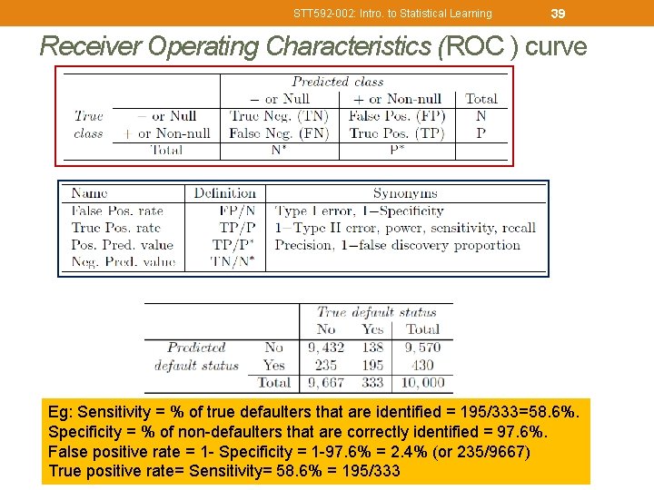
STT 592 -002: Intro. to Statistical Learning 35 Use 0. 2 as Threshold for Default • Now the total number of mistakes is 138+235 = 373 (3. 73% misclassification error rate) • But we miss-predicted 138/333 = 41. 4% of defaulters • Examine error rate with other thresholds: sensitivity and specificity. Eg: Sensitivity = % of true defaulters that are identified = 58. 6% (higher). Specificity = % of non-defaulters that are correctly identified = 97. 6%.

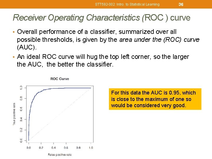
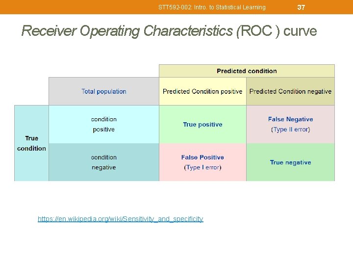
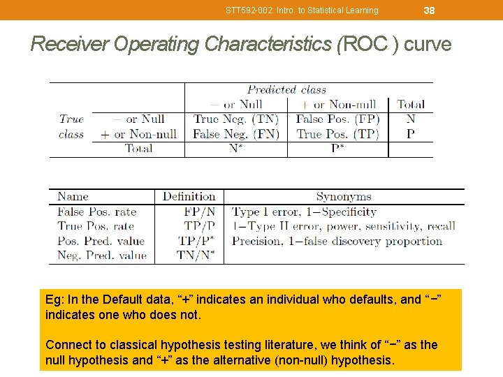
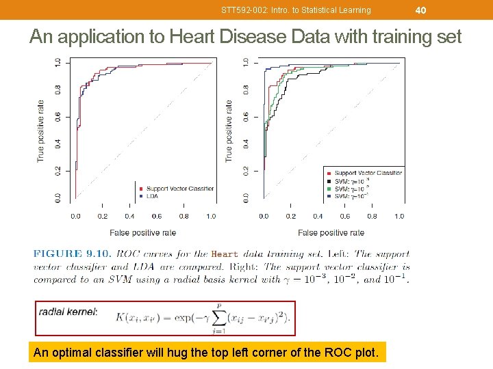
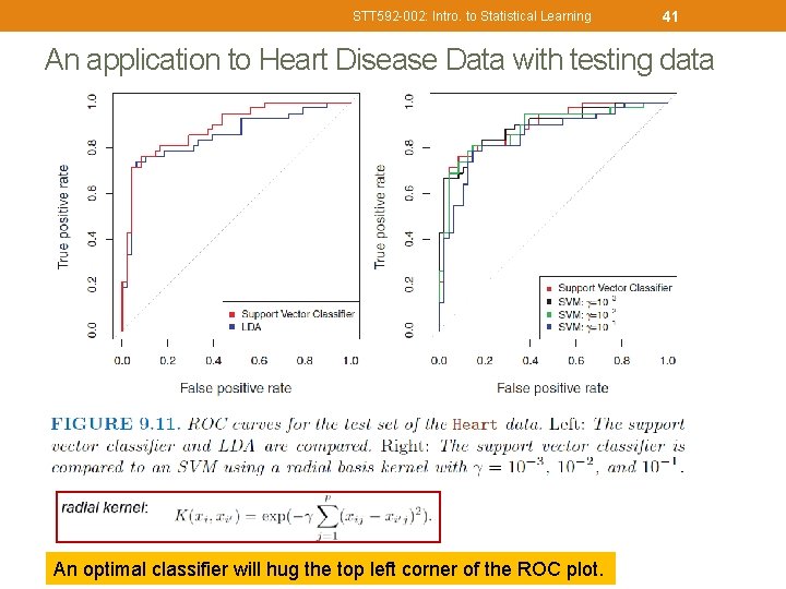
STT 592 -002: Intro. to Statistical Learning 36 Receiver Operating Characteristics (ROC ) curve • Overall performance of a classifier, summarized over all possible thresholds, is given by the area under the (ROC) curve (AUC). • An ideal ROC curve will hug the top left corner, so the larger the AUC, the better the classifier. For this data the AUC is 0. 95, which is close to the maximum of one so would be considered very good.

STT 592 -002: Intro. to Statistical Learning 37 Receiver Operating Characteristics (ROC ) curve https: //en. wikipedia. org/wiki/Sensitivity_and_specificity

STT 592 -002: Intro. to Statistical Learning 38 Receiver Operating Characteristics (ROC ) curve Eg: In the Default data, “+” indicates an individual who defaults, and “−” indicates one who does not. Connect to classical hypothesis testing literature, we think of “−” as the null hypothesis and “+” as the alternative (non-null) hypothesis.

STT 592 -002: Intro. to Statistical Learning 39 Receiver Operating Characteristics (ROC ) curve Eg: Sensitivity = % of true defaulters that are identified = 195/333=58. 6%. Specificity = % of non-defaulters that are correctly identified = 97. 6%. False positive rate = 1 - Specificity = 1 -97. 6% = 2. 4% (or 235/9667) True positive rate= Sensitivity= 58. 6% = 195/333

STT 592 -002: Intro. to Statistical Learning 40 An application to Heart Disease Data with training set An optimal classifier will hug the top left corner of the ROC plot.

STT 592 -002: Intro. to Statistical Learning 41 An application to Heart Disease Data with testing data An optimal classifier will hug the top left corner of the ROC plot.

STT 592 -002: Intro. to Statistical Learning 42 How to tune hyper-parameters in SVM • For cost C: • https: //stats. stackexchange. com/questions/31066/what-is- the-influence-of-c-in-svms-with-linear-kernel • • https: //www. csie. ntu. edu. tw/~cjlin/papers/guide. pdf