Please switch to slide show mode press F

Please switch to ‘slide show’ mode (press F 5)

This is a presentation by Roderick Hunt, Ric Colasanti & Andrew Askew University of Sheffield It is all about SAM A model involving self-assembling modular plants

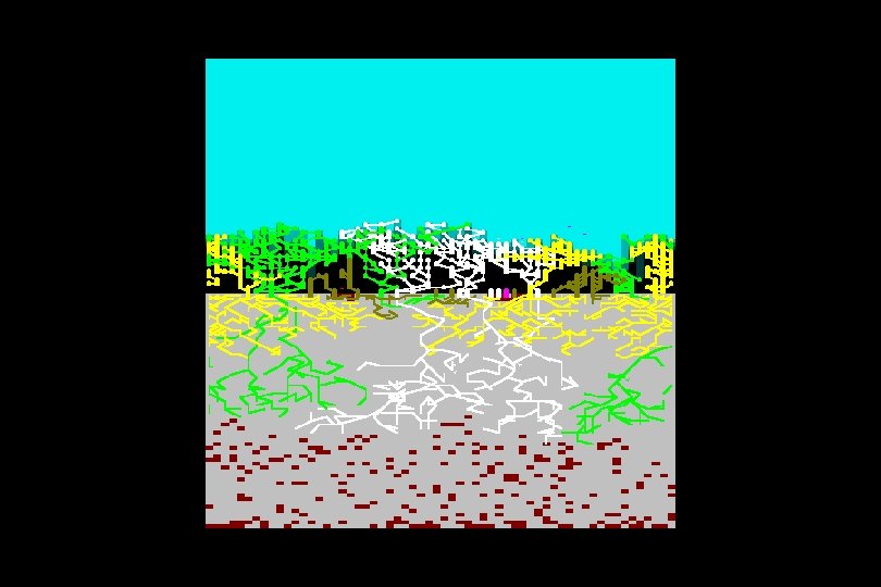
This is what a community of virtual plants looks like Contrasting tones show patches of resource

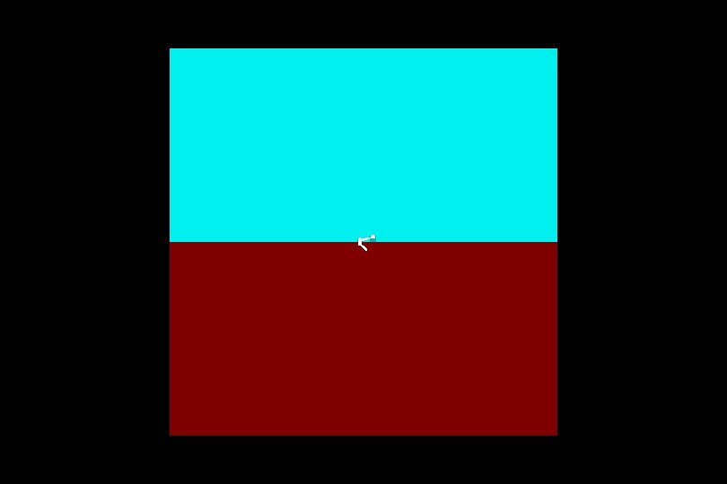
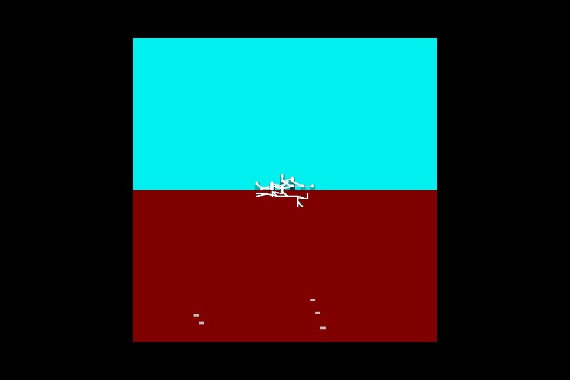
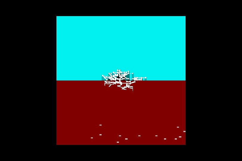
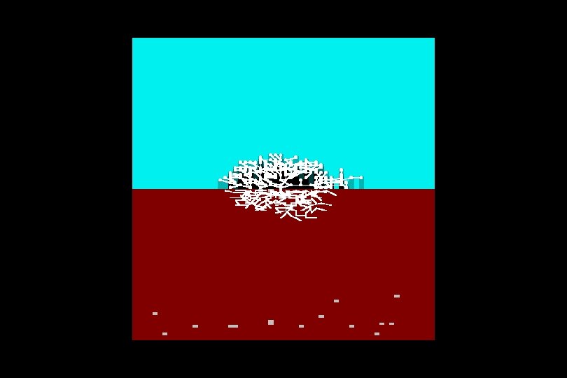
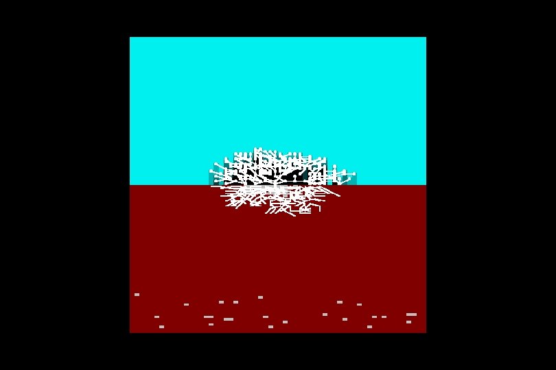
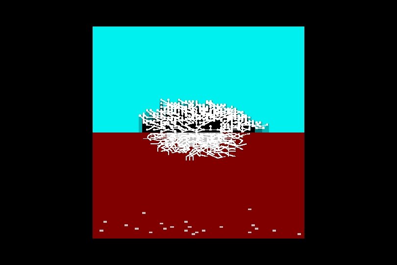
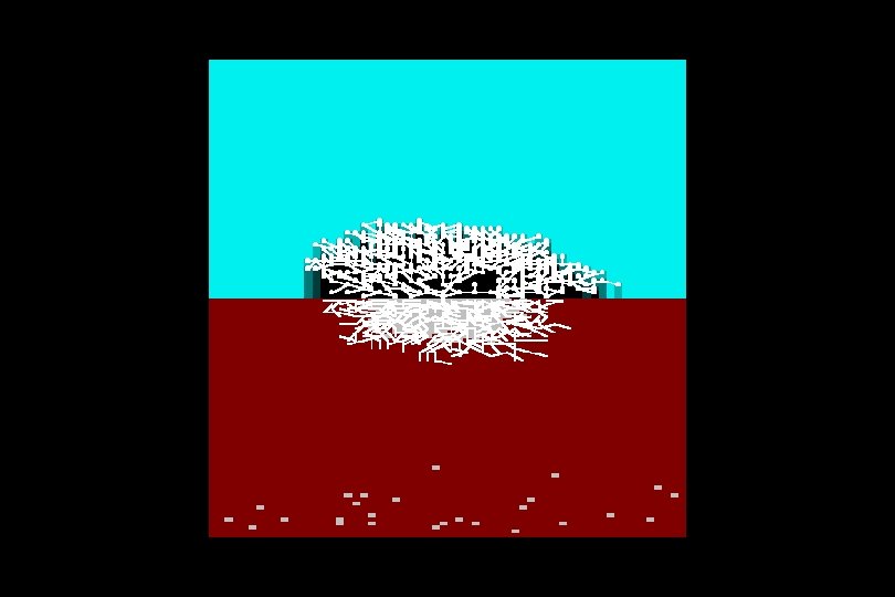
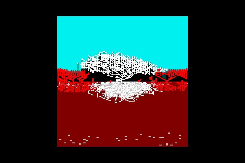
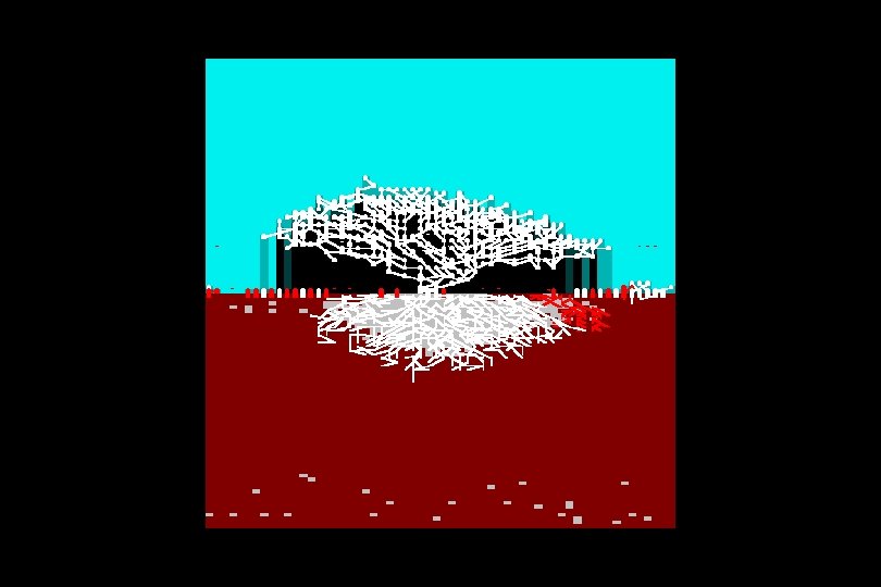
This is a single propagule of a virtual plant It is about to grow in a resource-rich above- and below-ground environment

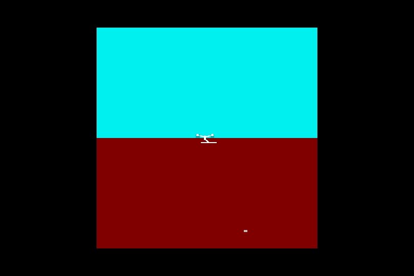
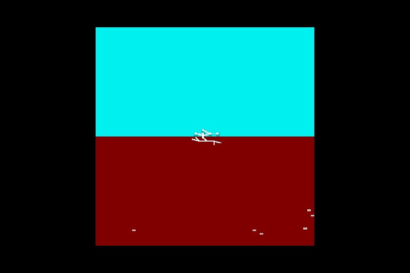
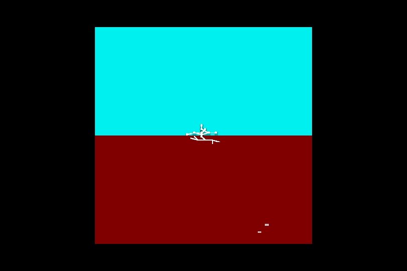
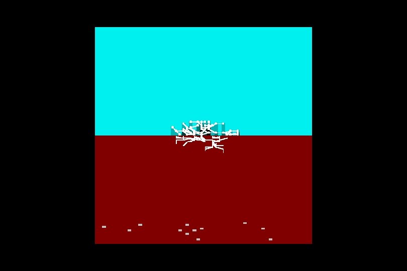
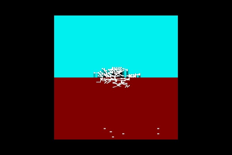
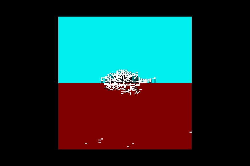
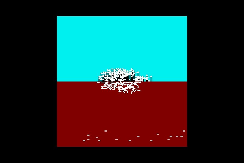
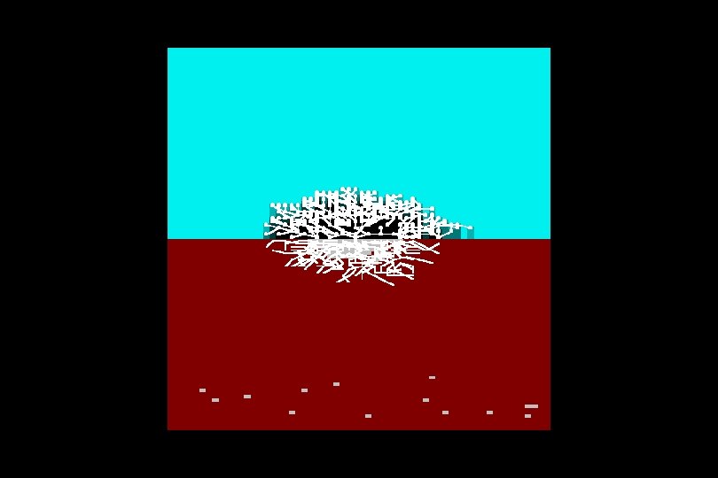
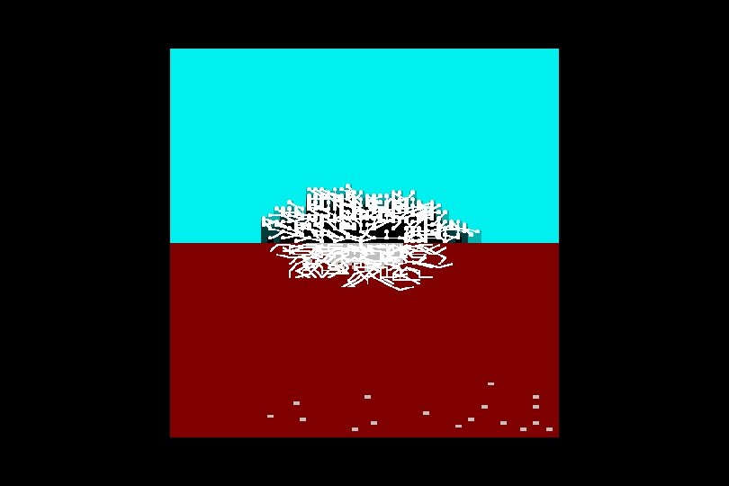
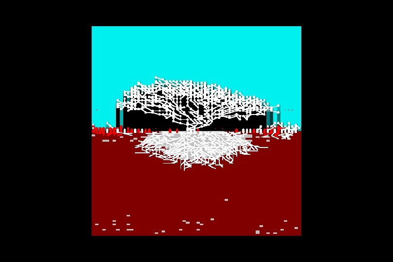
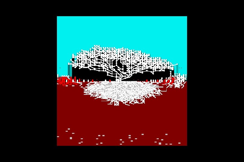
The plant has produced abundant growth aboveand below-ground and zones of resource depletion have appeared

Above-ground binary tree ( = shoot system) Each plant is structured like this A branching module Above-ground array Above-ground binary tree base module Below-ground array Below-ground binary tree base module This is only a diagram, not a painting ! An end module Below-ground binary tree ( = root system)

The end-modules capture resources: Light and carbon dioxide from aboveground Water and nutrients from belowground The branching (parent) modules can pass resources to any adjoining modules In this way whole plants can grow

The virtual plants interact with their environment (and with their neighbours) just like real ones do They possess most of the properties of real individuals and populations For example …

S-shaped growth curves

Partitioning towards the resourcepoorer half of the environment

Maintaining a functional equilibrium above-and belowground

Foraging towards resources in a heterogeneous environment

And when many plants are grown together in a dense population …

… they exhibit selfthinning but as the plants are 2 -dimensional the thinning slope is not – 3/2

All of these plants have the same specification (modular rulebase) But this specification can easily be changed if we want the plants to behave differently…

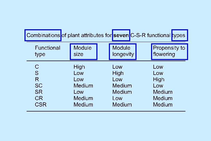
For example, we can recreate J P Grime’s system of C-S-R plant functional types For this, the specifications we need to change are those controlling morphology, physiology and reproductive behaviour …

With three levels possible in each of three traits, 27 simple functional types could be constructed However, we model only 7 types; the other 20 include Darwinian Demons that do not respect evolutionary tradeoffs

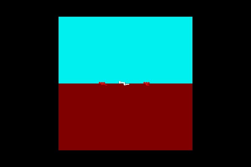
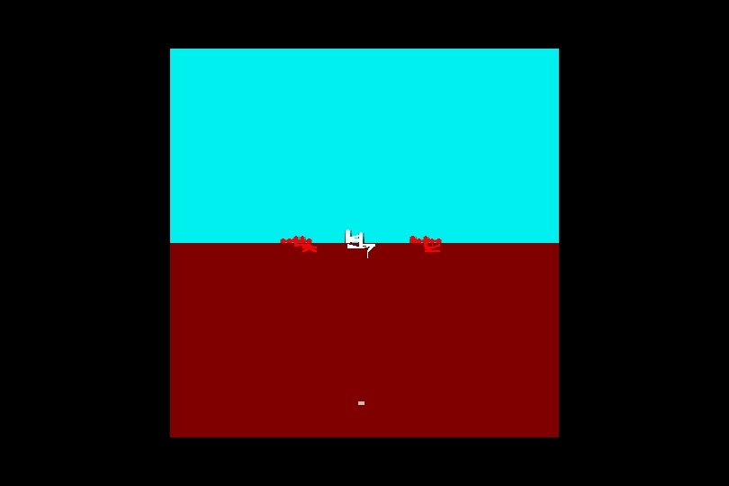
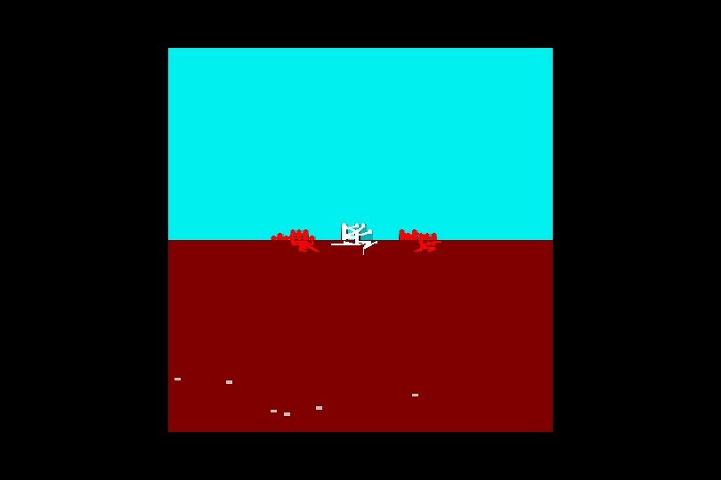
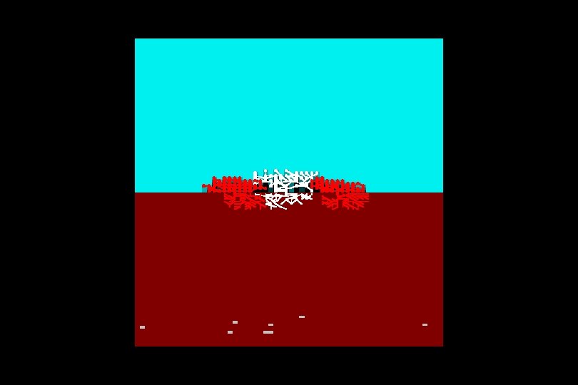
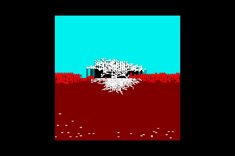
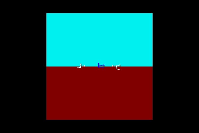
Let us see some competition between different types of plant Initially we will use only two types …

Small size, rapid growth and fast reproduction Medium size, moderately fast in growth and reproduction

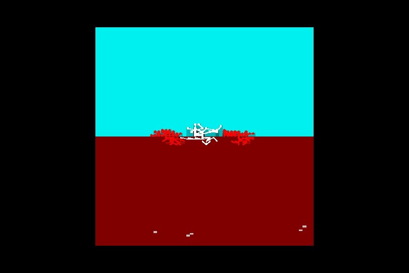
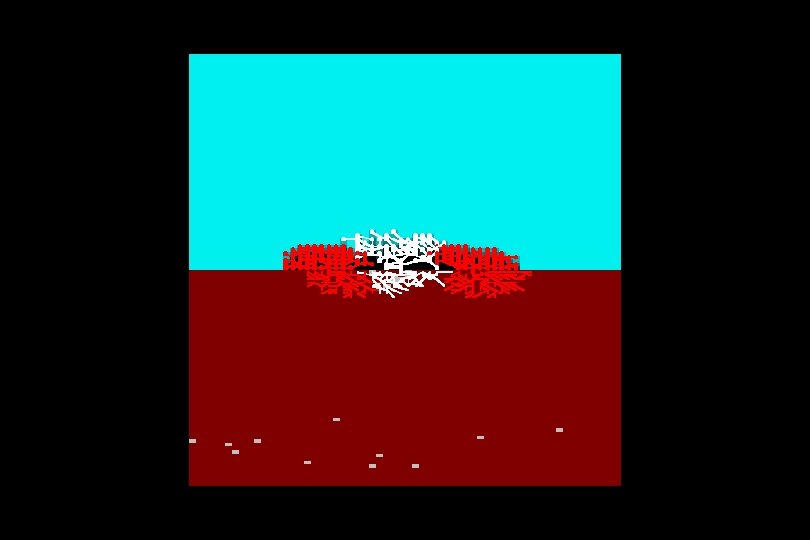
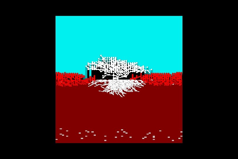
(Red enters its 2 nd generation)

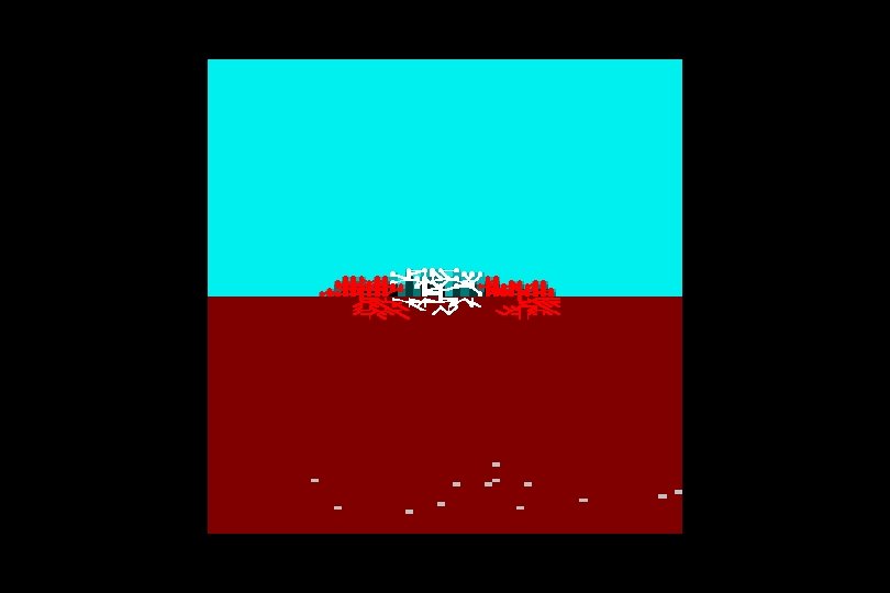
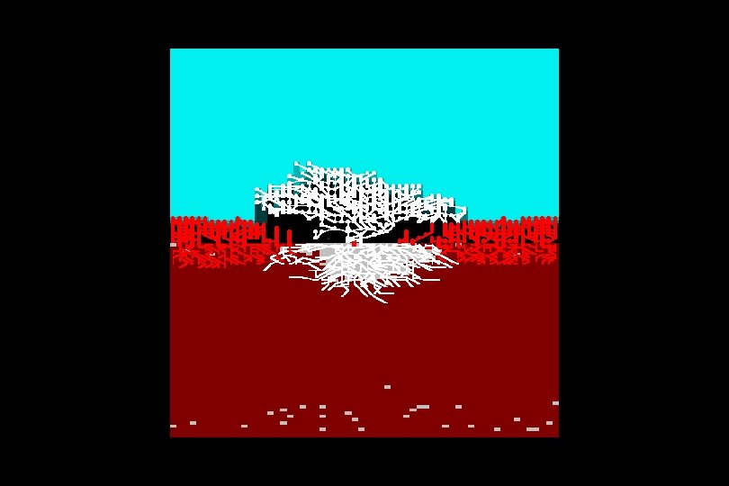
White has won !

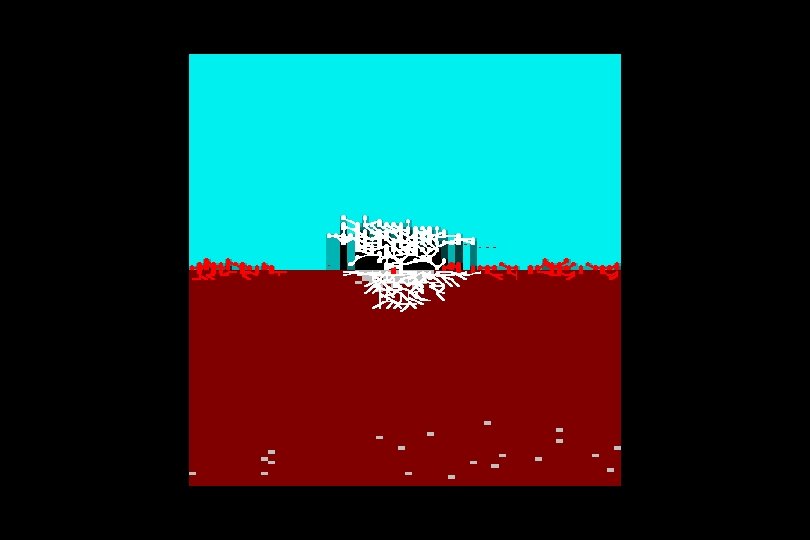
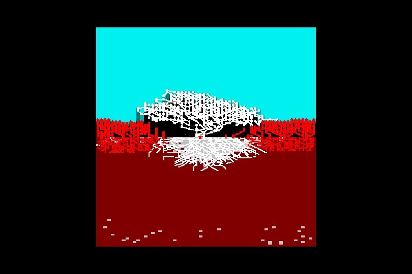
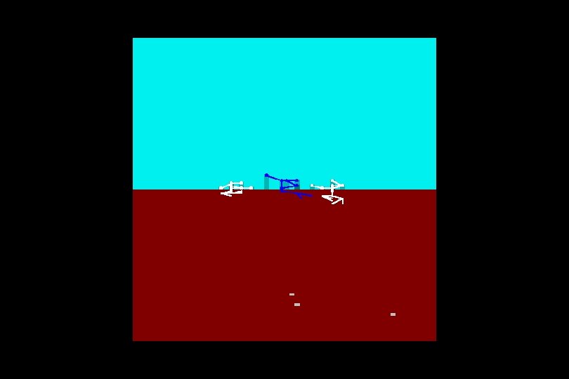
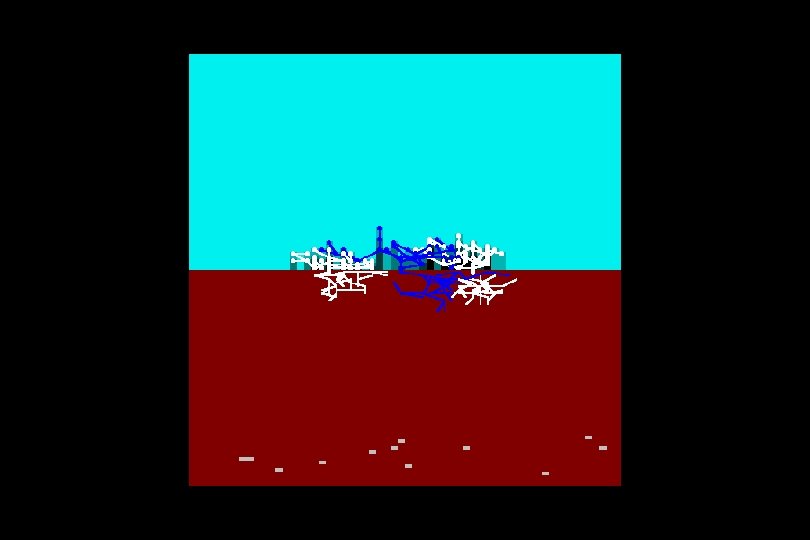
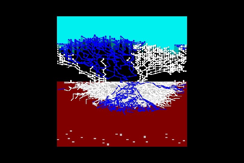
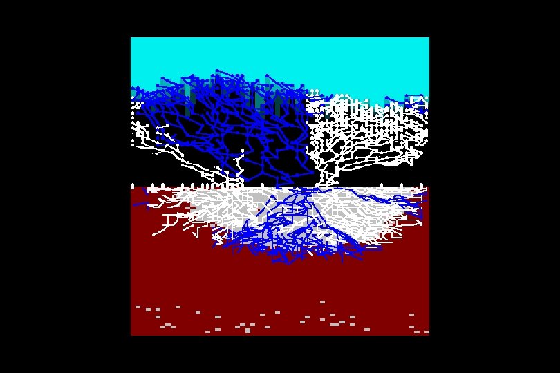
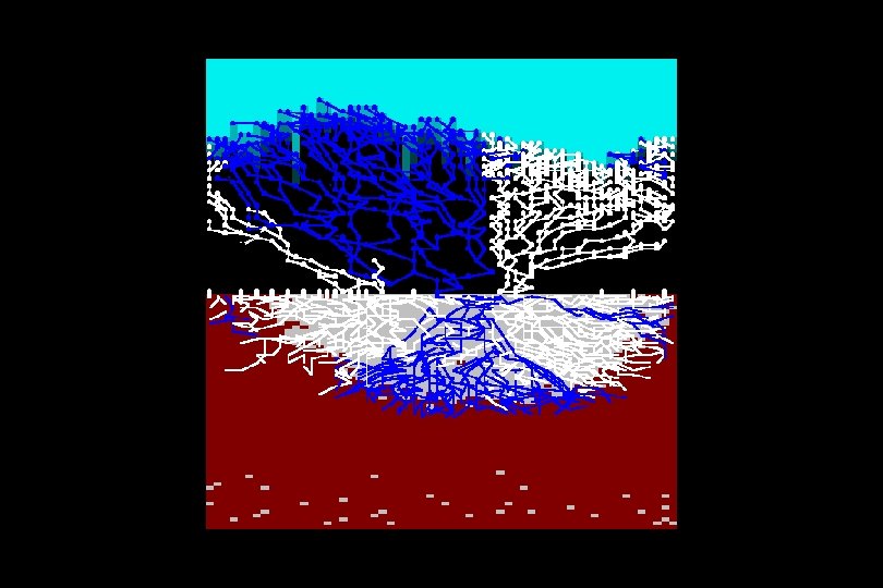
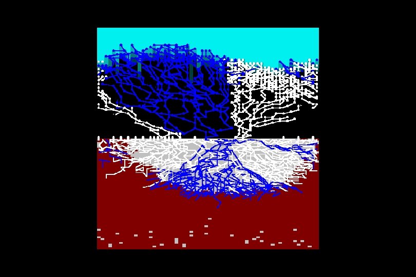
Now let us see if white always wins This time, its competitor is rather different …

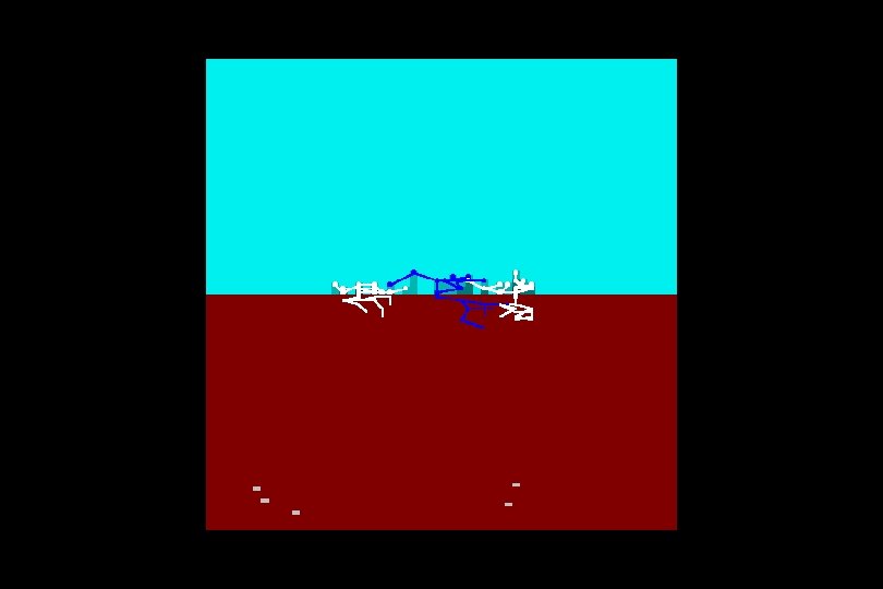
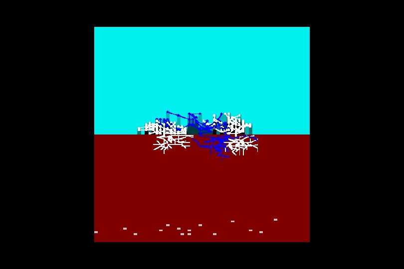
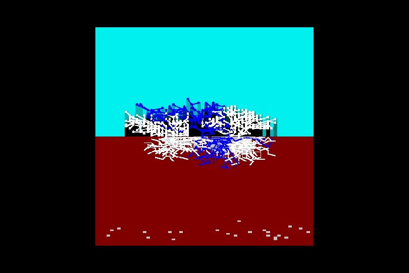
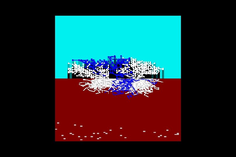
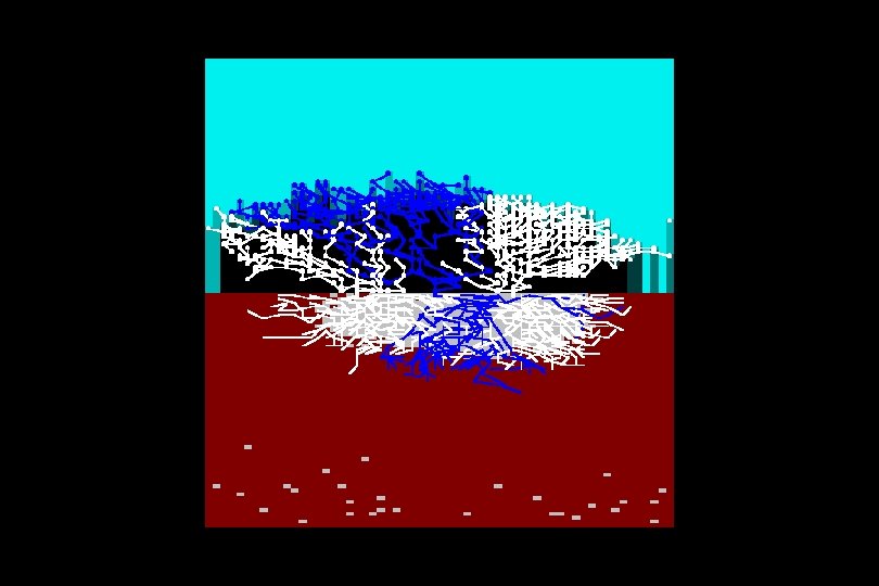
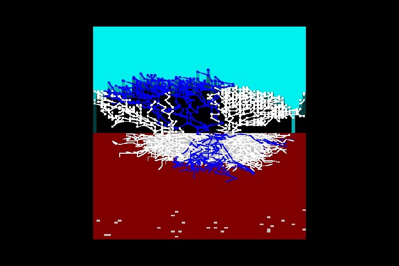
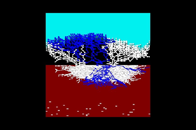
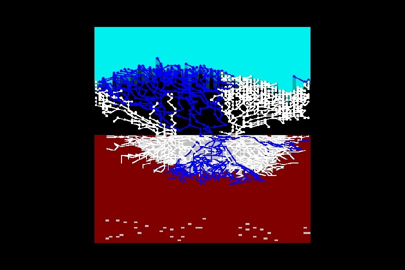
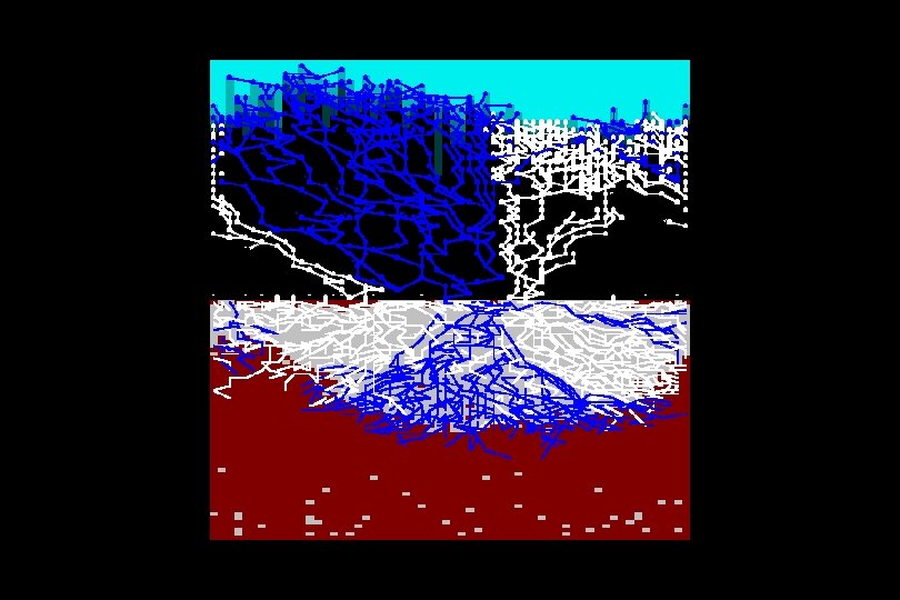
Medium size, moderately fast in growth and reproduction Large size, very fast growing, slow reproductio n

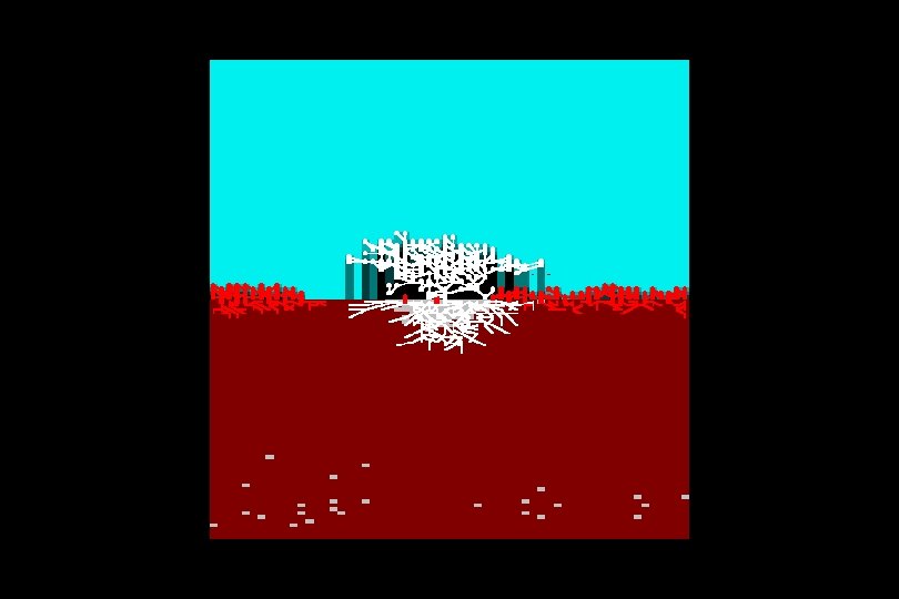
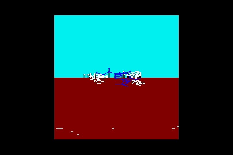
The huge blue type has outcompeted both of the white plants, both above- and belowground And the simulation has run out of space …

So competition can be demonstrated realistically … … but most real communities involve more than two types of plant

We need seven functional types to cover the entire range of variation shown by herbaceous plant life To a first approximation, these seven types can simulate complex community processes very realistically

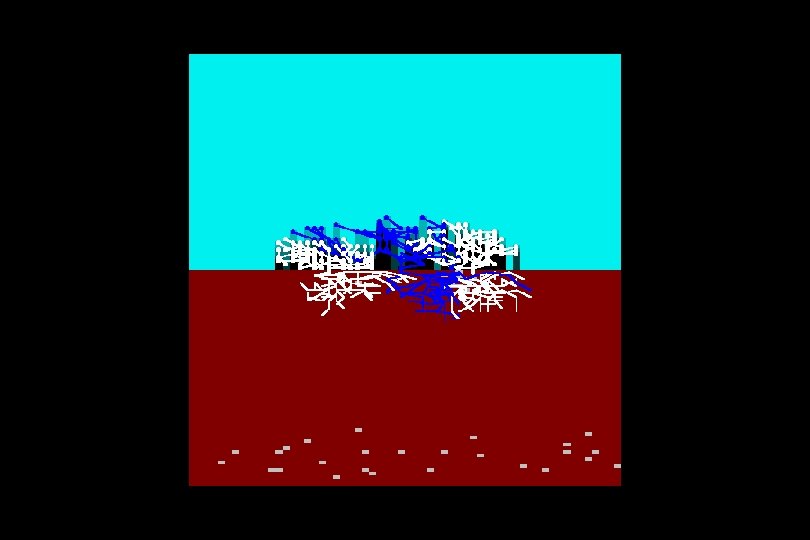
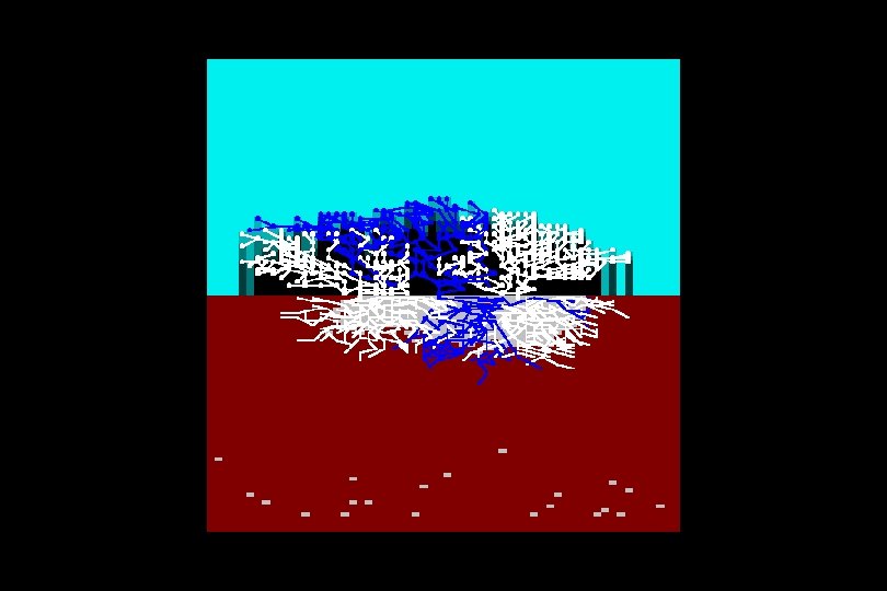
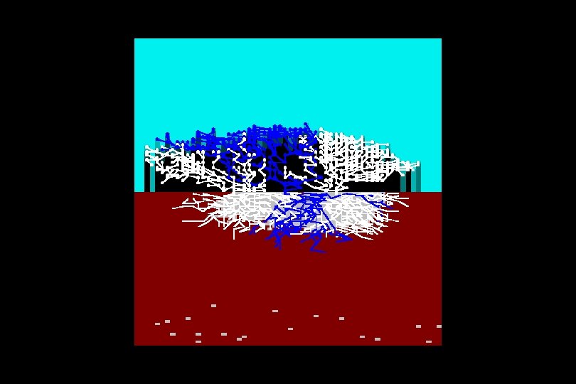
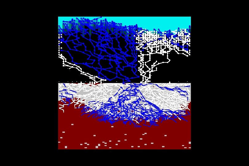
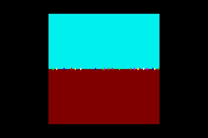
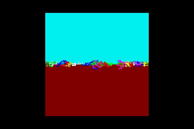
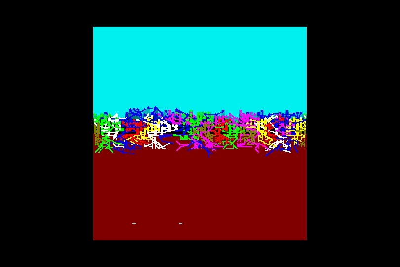
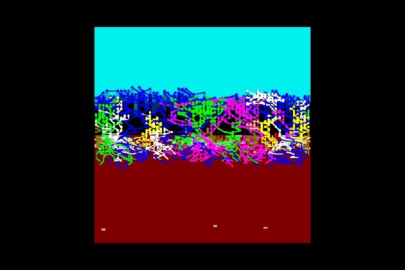
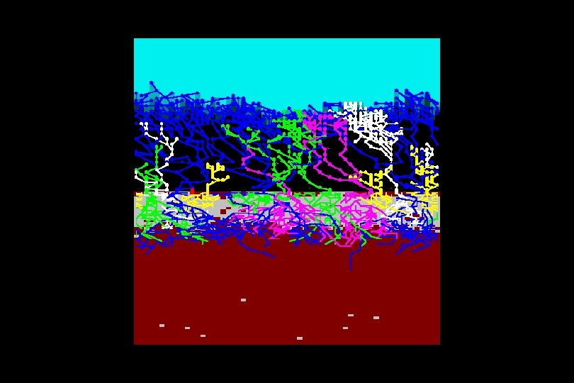
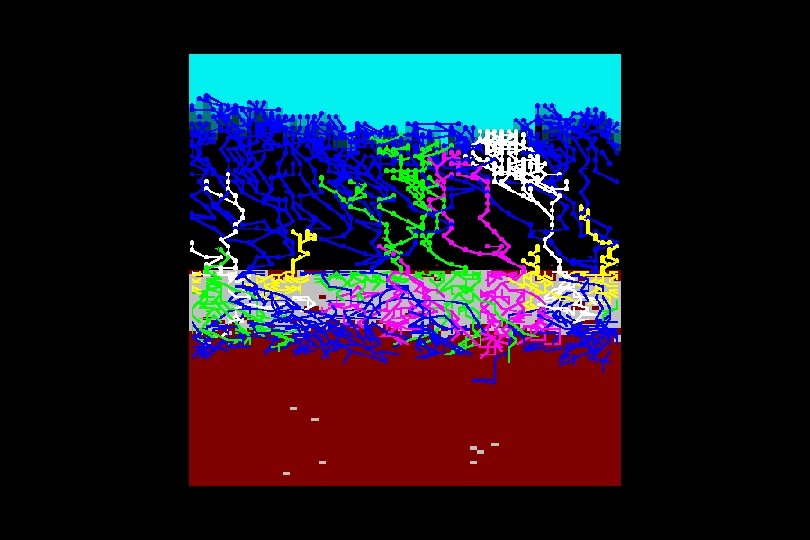
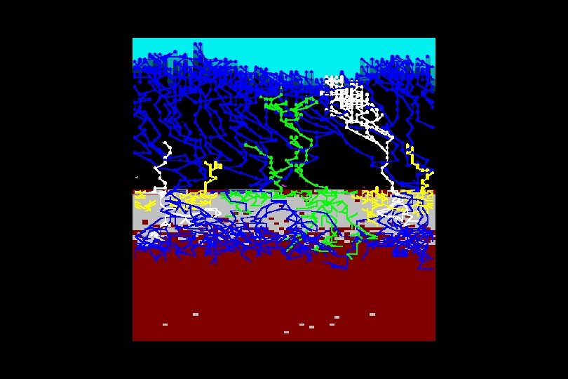
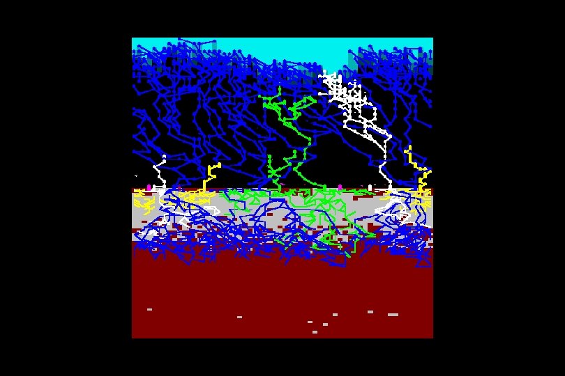
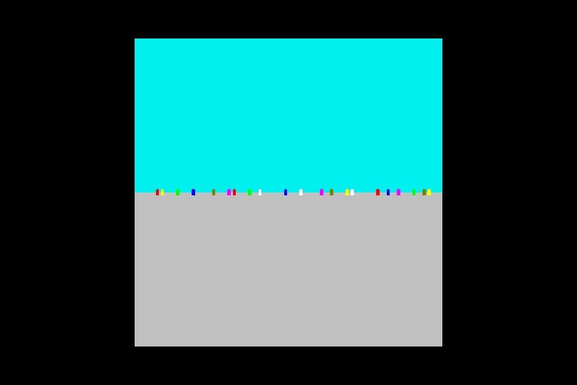
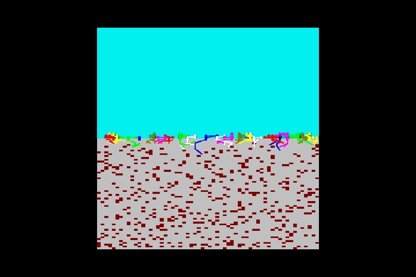
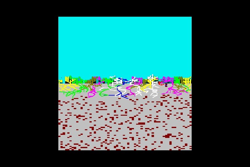
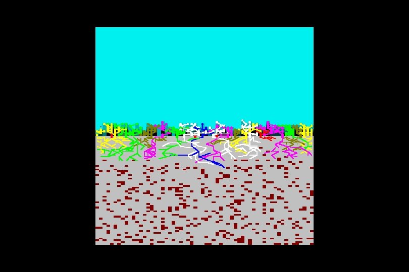
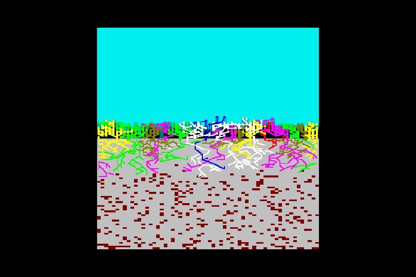
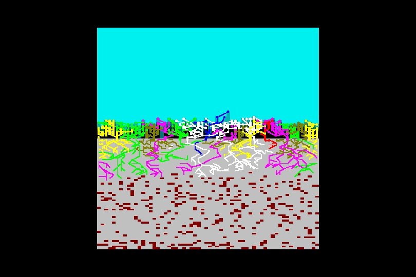
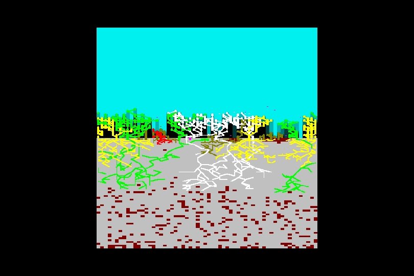
For example, an equal mixture of all seven types can be grown together … … in an environment which has high levels of resource, both above- and below-ground

The blue type has eliminated almost everything except white and green types And the simulation has almost run out of space again …

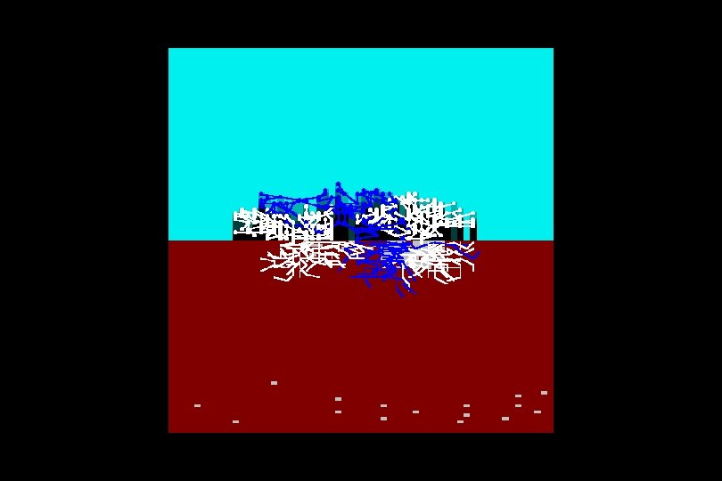
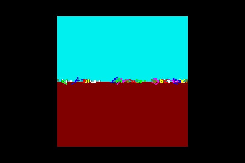
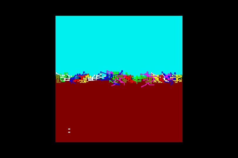
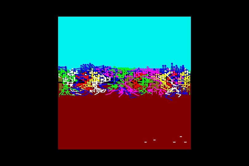
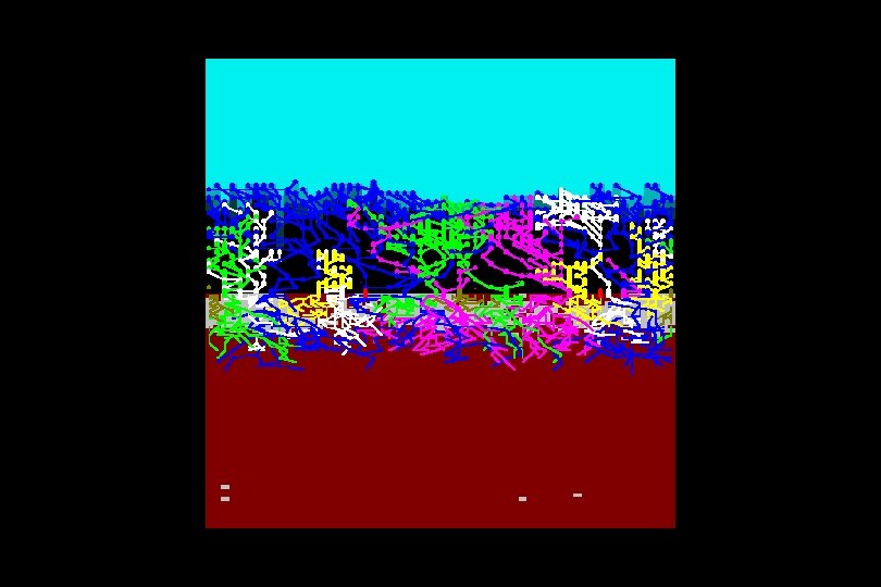
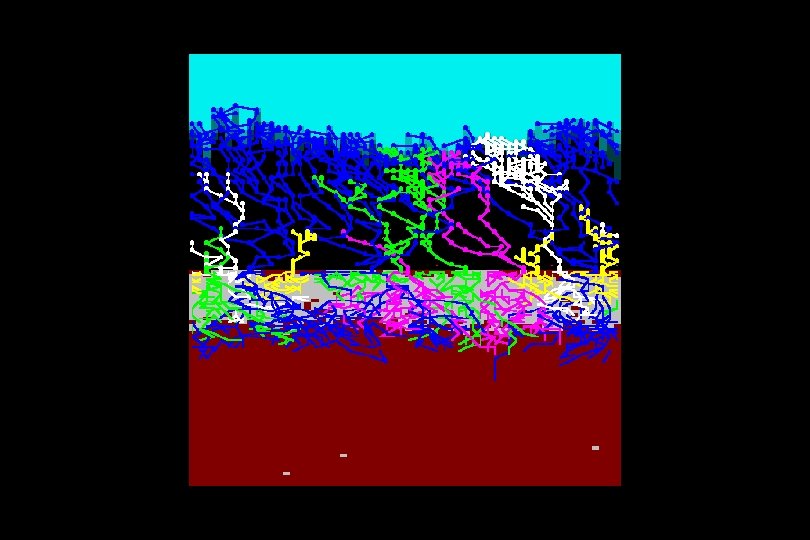
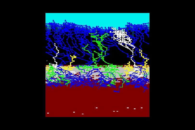
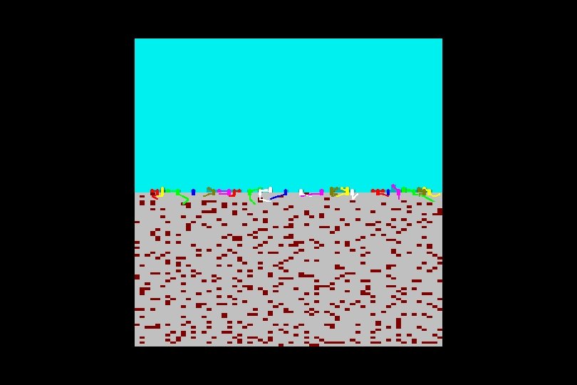
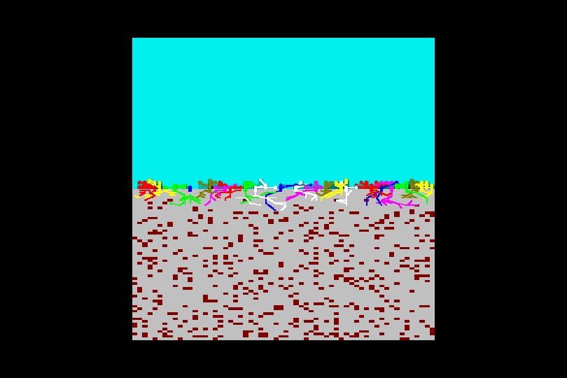
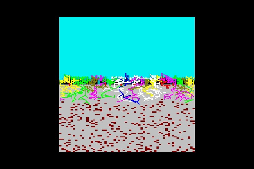
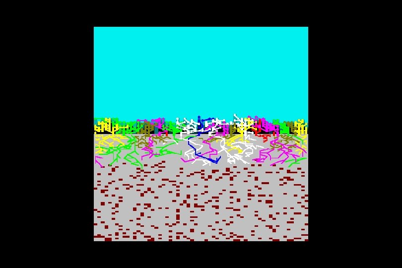
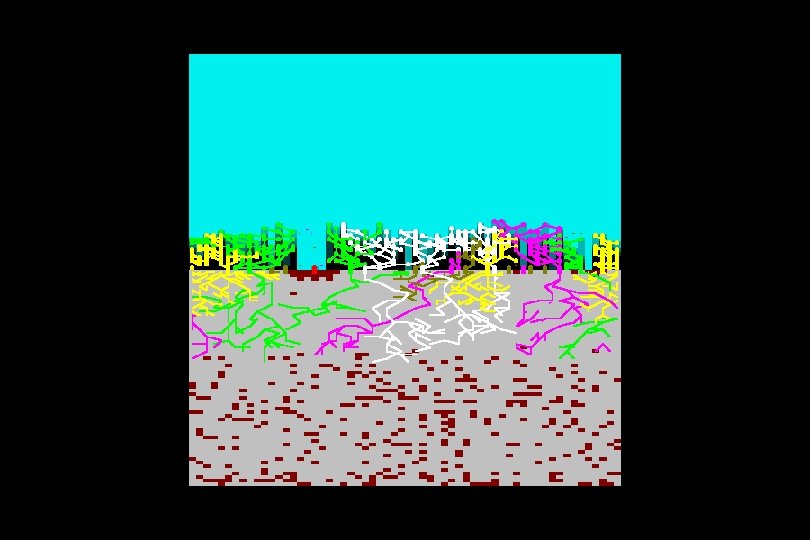
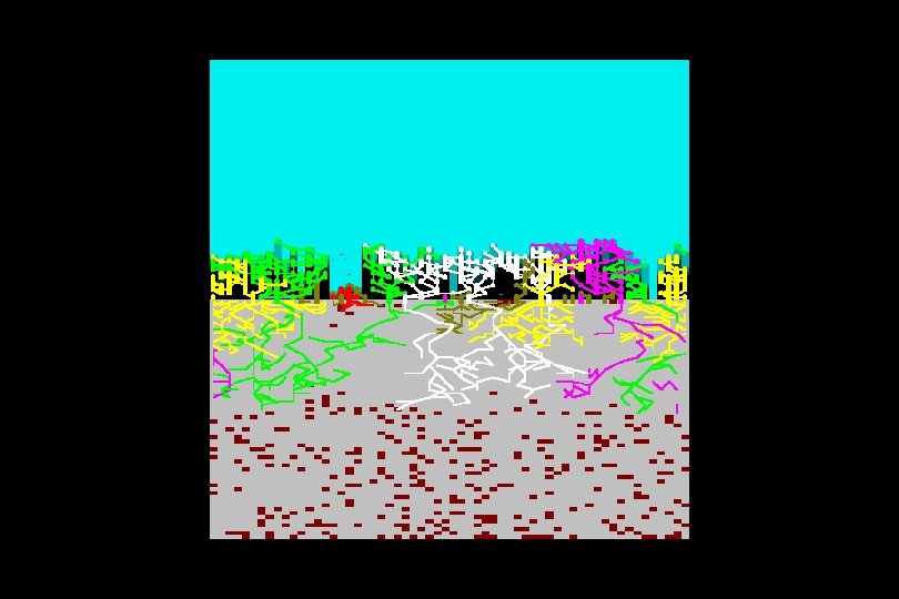
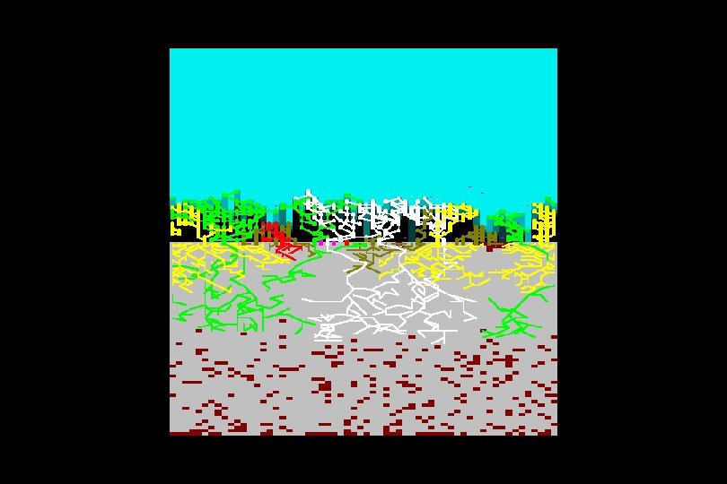
Now we grow the equal mixture of all seven types again … … but this time the environment has low levels of mineral nutrient resource, as indicated by the many grey cells

(a gap has appeared here)

(red tries to colonize)

(but is unsuccessful)

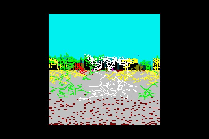
White, green and yellow finally predominate … … blue is nowhere to be seen … … and total biomass is much reduced

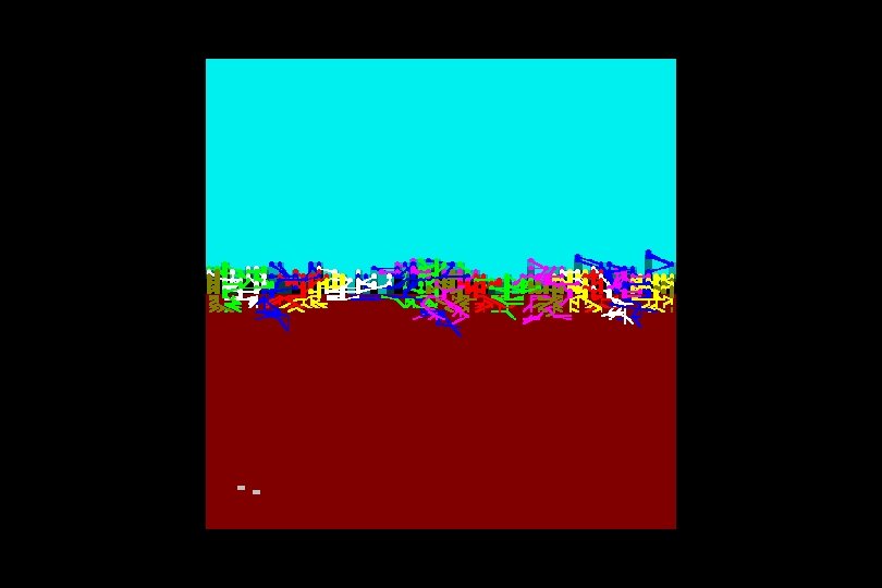
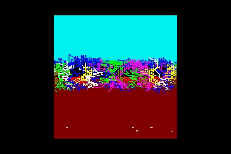
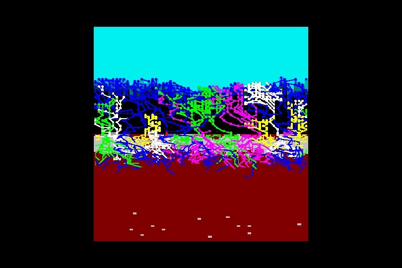
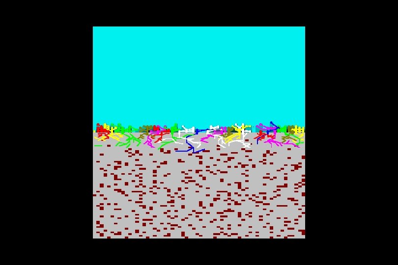
Environmental gradients can be simulated by increasing resource levels in steps Whittaker-type niches then appear for contrasting plant types within these gradients

(types)

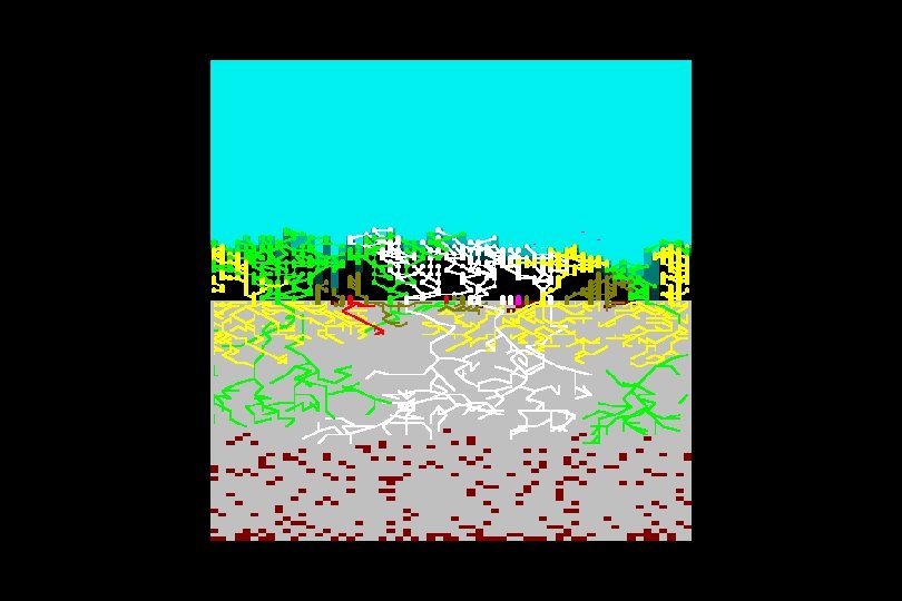
Next we grow the equal mixture of all seven types again … … but this time under an environmental gradient of increasing mineral nutrient resource

Greatest biodiversity is at intermediate stress

Now, environmental disturbance can be defined as ‘removal of biomass after it has been created’ For example, grazing, cutting, burning and trampling are all forms of disturbance

In our model, ‘trampling’ can be applied simply by removing shoot material from certain sizes of patch at certain intervals of time and in a certain number of places Other forms of disturbance can be simulated by varying each of these factors

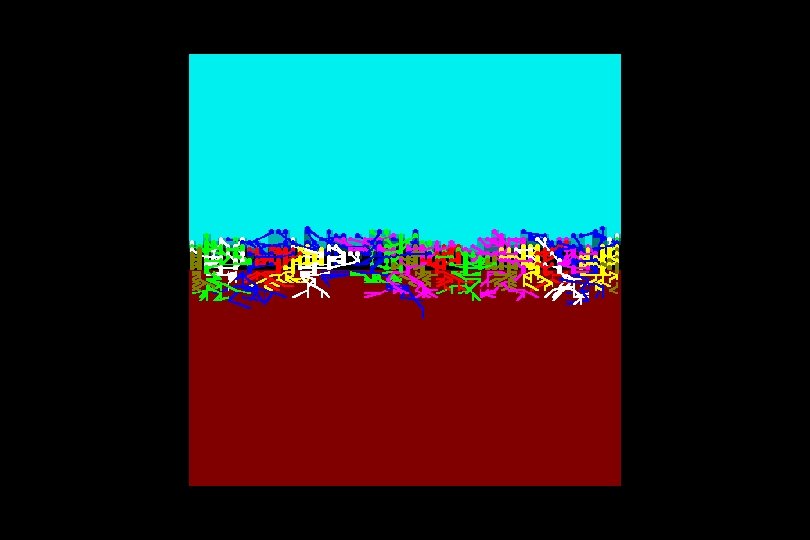
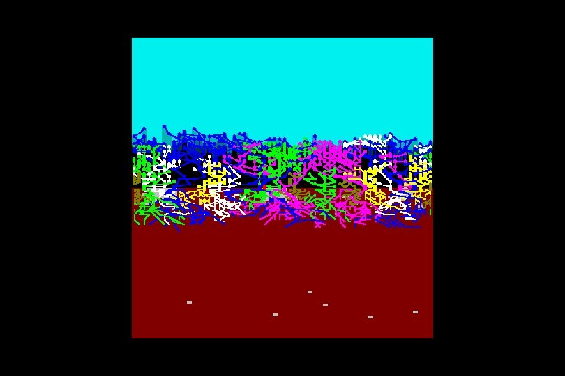
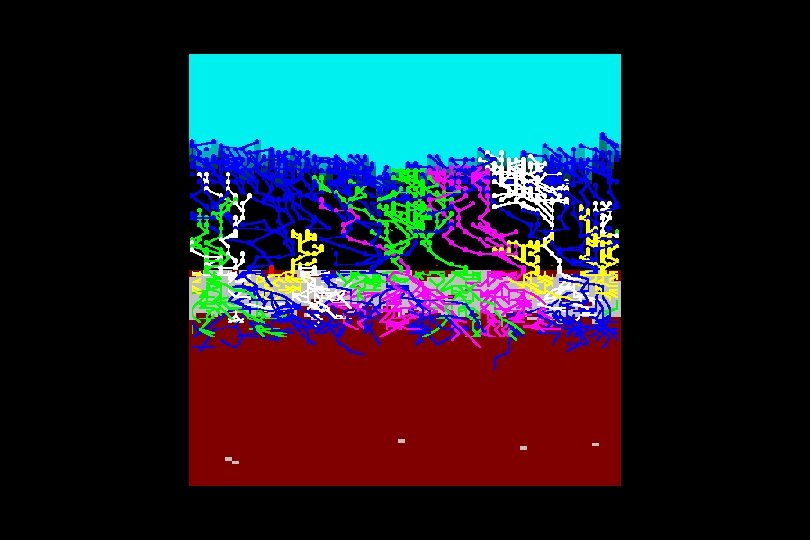
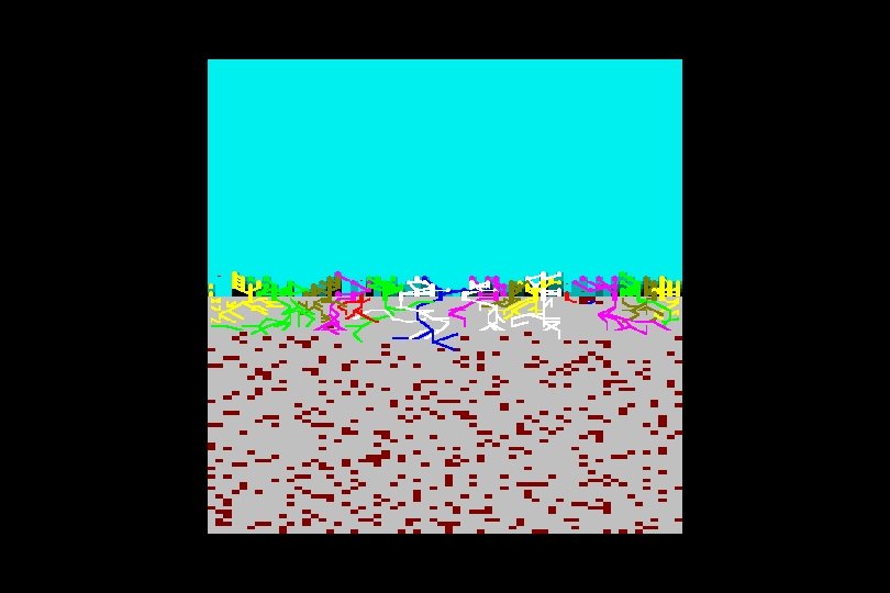
So we grow the equal mixture of all seven types again … … but this time under an environmental gradient of increasing ‘trampling’ disturbance

Greatest biodiversity is at intermediate disturbance … … but the final number of types is low

Environmental stress and disturbance can, of course, be applied together This can be done in all forms and combinations

Again we grow the equal mixture of all seven types … … but with one of seven levels of stress and seven levels of disturbance in all factorial combinations

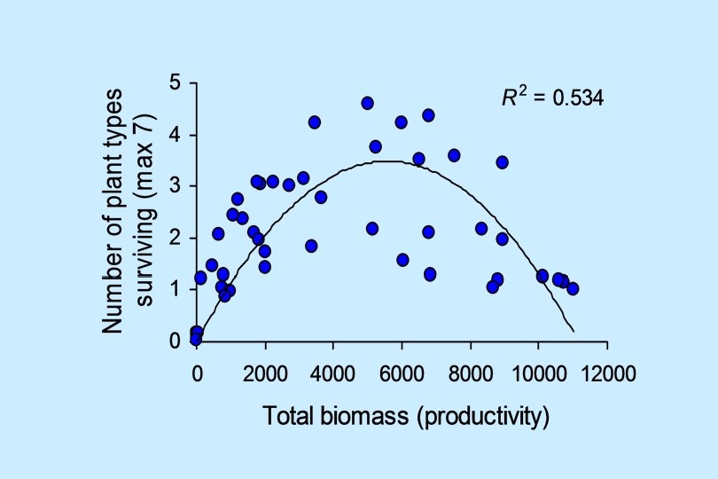
Greatest biodiversity is at intermediate productivity

The biomass-driven humpbacked relationship is one of the highestlevel properties that real plant communities possess Yet it emerges from the model solely because of the resource-capturing activity of modules in the selfassembling plants