Perceptron This is convolution v v v Shared


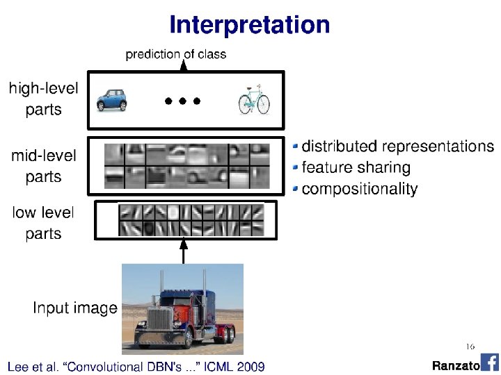


 Input")

![Alex. Net diagram (simplified) [Krizhevsky et al. 2012] Input size 227 x 3 227](https://slidetodoc.com/presentation_image_h/30937a2fbb466d63dd36b5156ca3e323/image-20.jpg "Alex. Net diagram (simplified) [Krizhevsky et al. 2012] Input size 227 x 3 227")


 …is a ‘fully connected’ neural network with nonlinear activation functions. ‘Feed-forward’")


")


… Three different kernels trained to fire")


 x")
 x")
 f(x) x")
 x")
 x")
 x")


 Model parameters")


: “Squashes\" a C-dimensional")


 as training data point is")

 optimum Wikipedia")


![Data fitting problem [Nielson]](https://slidetodoc.com/presentation_image_h/30937a2fbb466d63dd36b5156ca3e323/image-100.jpg "Data fitting problem [Nielson]")


![Regularization: • [Nielson]](https://slidetodoc.com/presentation_image_h/30937a2fbb466d63dd36b5156ca3e323/image-103.jpg "Regularization: • [Nielson]")

![Regularization • Normal cross-entropy loss (binary classes) Regularization term [Nielson]](https://slidetodoc.com/presentation_image_h/30937a2fbb466d63dd36b5156ca3e323/image-105.jpg "Regularization • Normal cross-entropy loss (binary classes) Regularization term [Nielson]")


![Regularization: Dropout [Nielson]](https://slidetodoc.com/presentation_image_h/30937a2fbb466d63dd36b5156ca3e323/image-108.jpg "Regularization: Dropout [Nielson]")


- Slides: 110
Perceptron: This is convolution!
v v v Shared weights v
Filter = ‘local’ perceptron. Also called kernel.
Yann Le. Cun’s MNIST CNN architecture
DEMO http: //scs. ryerson. ca/~aharley/vis/conv/ Thanks to Adam Harley for making this. More here: http: //scs. ryerson. ca/~aharley/vis
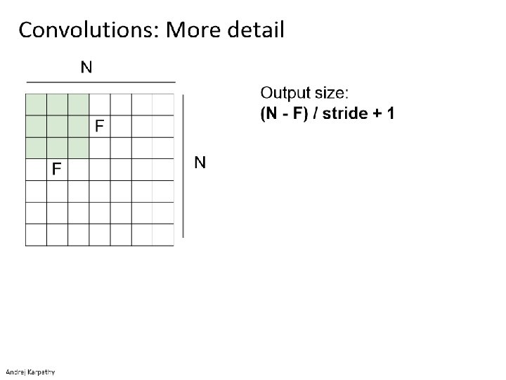
Think-Pair-Share Input size: 96 x 3 Kernel size: 5 x 3 Stride: 1 Max pooling layer: 4 x 4 Input size: 96 x 3 Kernel size: 3 x 3 Stride: 3 Max pooling layer: 8 x 8 Output feature map size? a) 5 x 5 b) 22 x 22 c) 23 x 23 d) 24 x 24 e) 25 x 25 Output feature map size? a) 2 x 2 b) 3 x 3 c) 4 x 4 d) 5 x 5 e) 12 x 12
Our connectomics diagram Auto-generated from network declaration by nolearn (for Lasagne / Theano) Input 75 x 4 Conv 1 3 x 3 x 4 64 filters Conv 2 3 x 3 x 64 48 filters Max pooling 2 x 2 per filter Conv 3 3 x 3 x 48 48 filters Conv 4 3 x 3 x 48 48 filters Max pooling 2 x 2 per filter
Reading architecture diagrams Layers - Kernel sizes - Strides - # channels - # kernels - Max pooling
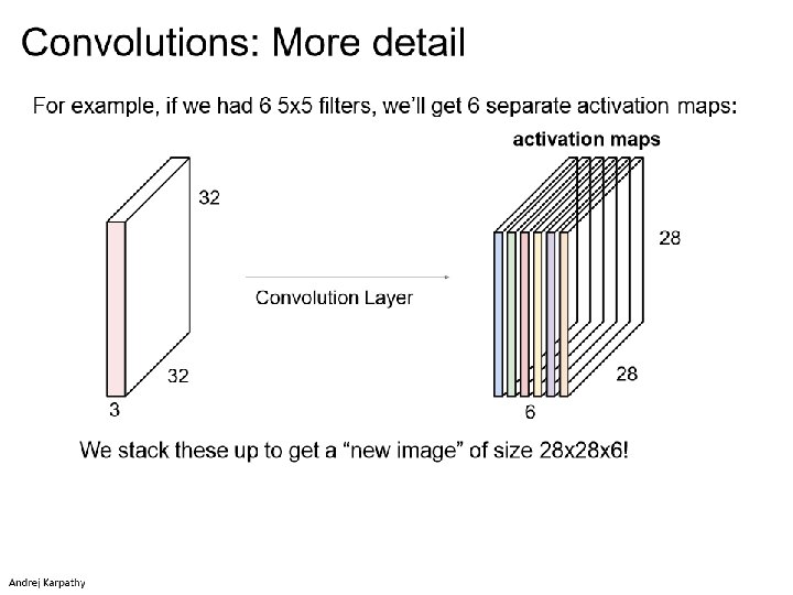
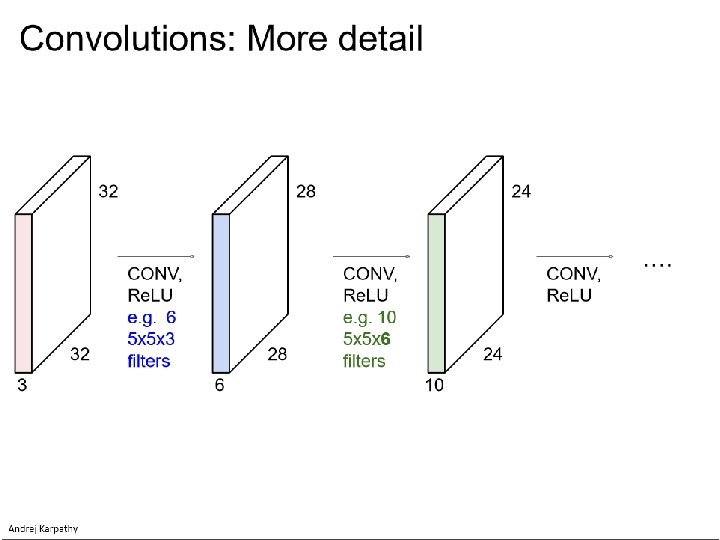
Alex. Net diagram (simplified) [Krizhevsky et al. 2012] Input size 227 x 3 227 3 x 3 Stride 2 227 Conv 1 11 x 3 Stride 4 96 filters Conv 2 5 x 96 Stride 1 256 filters 3 x 3 Stride 2 Conv 3 3 x 256 Stride 1 384 filters Conv 4 3 x 3 x 192 Stride 1 256 filters
Wait, why isn’t it called a correlation neural network? It could be. Deep learning libraries implement correlation. Correlation relates to convolution via a 180 deg rotation of the kernel. When we learn kernels, we could easily learn them flipped. Associative property of convolution ends up not being important to our application, so we just ignore it. [p. 323, Goodfellow]
What does it mean to convolve over greater-than-first-layer hidden units?
Yann Le. Cun’s MNIST CNN architecture
Multi-layer perceptron (MLP) …is a ‘fully connected’ neural network with nonlinear activation functions. ‘Feed-forward’ neural network Nielson
Does anyone pass along the weight without an activation function? No – this is linear chaining. Input vector Output vector
Does anyone pass along the weight without an activation function? No – this is linear chaining. Input vector Output vector
Are there other activation functions? Yes, many. As long as: - Activation function s(z) is well-defined as z -> -∞ and z -> ∞ - These limits are different Then we can make a step! [Think visual proof] It can be shown that it is universal for function approximation.
Activation functions: Rectified Linear Unit • Re. LU
Cyh 24 - http: //prog 3. com/sbdm/blog/cyh_24
Rectified Linear Unit Ranzato
What is the relationship between SVMs and perceptrons? SVMs attempt to learn the support vectors which maximize the margin between classes.
What is the relationship between SVMs and perceptrons? SVMs attempt to learn the support vectors which maximize the margin between classes. A perceptron does not. Both of these perceptron classifiers are equivalent. ‘Perceptron of optimal stability’ is used in SVM: Perceptron + optimal stability + kernel trick = foundations of SVM
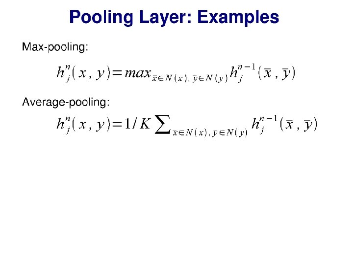
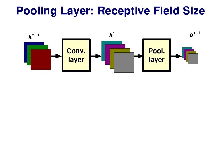
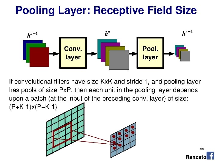
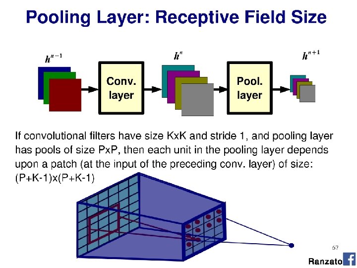
Why is pooling useful again? What kinds of pooling operations might we consider?
By pooling responses at different locations, we gain robustness to the exact spatial location of image features. Useful for classification, when I don’t care about _where_ I ‘see’ a feature! Pooling layer output Convolutional layer output
Pooling is similar to downsampling …but on feature maps, not the input! …except sometimes we don’t want to blur, as other functions might be better for classification.
Max pooling Wikipedia
OK, so what about invariances? What about translation, scale, rotation? Convolution is translation equivariant (‘shift-equivariant’) – we could shift the image and the kernel would give us a corresponding (‘equal’) shift in the feature map. But! If we rotated or scaled the input, the same kernel would give a different response. Pooling lets us aggregate (avg) or pick from (max) responses, but the kernels themselves must be trained and so learn to activate on scaled or rotated instances of the object.
If we max pooled over depth (# kernels)… Three different kernels trained to fire on different rotations of ‘ 5’. Fig 9. 9, Goodfellow et al. [the book]
I’ve heard about many more terms of jargon! Skip connections Residual connections Batch normalization …we’ll get to these in a little while.
Training Neural Networks Learning the weight matrices W
Gradient descent f(x) x
General approach Pick random starting point. f(x) x
General approach Compute gradient at point (analytically or by finite differences) f(x) x
General approach Move along parameter space in direction of negative gradient f(x) x
General approach Move along parameter space in direction of negative gradient. f(x) x
General approach Stop when we don’t move any more. f(x) x
Gradient descent Optimizer for functions. Guaranteed to find optimum for convex functions. • Non-convex = find local optimum. • Most vision problems aren’t convex. f(x) x Works for multi-variate functions. • Need to compute matrix of partial derivatives (“Jacobian”)
Why would I use this over Least Squares? If my function is convex, why can’t I just use linear least squares? Analytic solution = normal equations You can, yes.
Why would I use this over Least Squares? But now imagine that I have 1, 000 data points. Matrices are _huge_. Even for convex functions, gradient descent allows me to iteratively solve the solution without requiring very large matrices. We’ll see how.
Train NN with Gradient Descent •
Train NN with Gradient Descent Loss function (Evaluate NN on training data) Model parameters (perceptron weights)
utput
What is an appropriate loss? •
Classification as probability Special function on last layer - ‘Softmax’ σ(): “Squashes" a C-dimensional vector O of arbitrary real values to a C-dimensional vector σ(O) of real values in the range (0, 1) that add up to 1. Turns the output into a probability distribution on classes.
Classification as probability Softmax example: “Squashes" a C-dimensional vector O of arbitrary real values to a C-dimensional vector σ(O) of real values in the range (0, 1) that add up to 1. Turns the output into a probability distribution on classes. Output from perceptron layer ‘distance from class boundary’ O = [2. 0, 0. 7, 0. 2, -0. 3, -0. 6, -2. 5] σ(O) = [0. 616, 0. 168, 0. 102, 0. 061, 0. 046, 0. 007]
Softmax utput Softmax
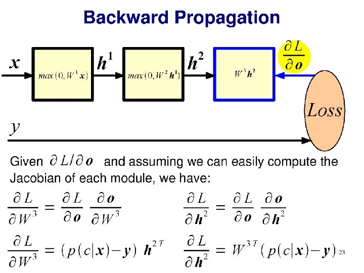
Cross-entropy loss function Negative log-likelihood • Measures difference between L predicted and training probability distributions (see Project 4 for more details) • Is it a good loss? • Differentiable • Cost decreases as probability increases p(cj|x)
Softmax utput
Training Learning consists of minimizing the loss wrt. parameters over the whole training set.
Training Learning consists of minimizing the loss wrt. parameters over the whole training set.
Softmax
Softmax
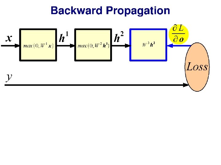
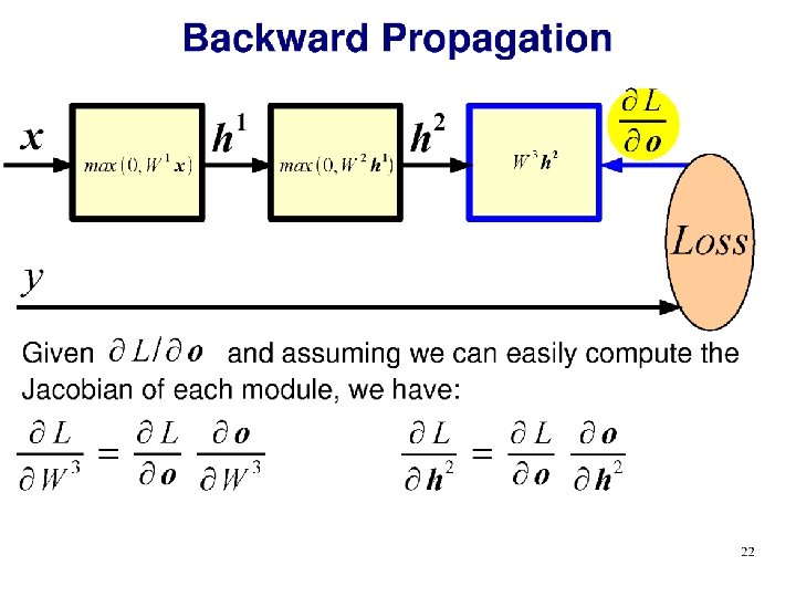
Derivative of loss wrt. softmax
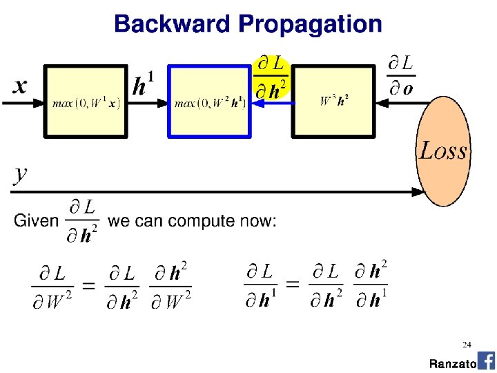
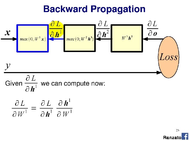
<- Chain rule from calculus
But the Re. LU is not differentiable at 0! Right. Fudge! - ‘ 0’ is the best place for this to occur, because we don’t care about the result (it is no activation). - ‘Dead’ perceptrons - Re. LU has unbounded positive response: - Potential faster convergence / overstep
Optimization demo • http: //www. emergentmind. com/neural-network • Thank you Matt Mazur
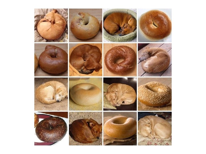
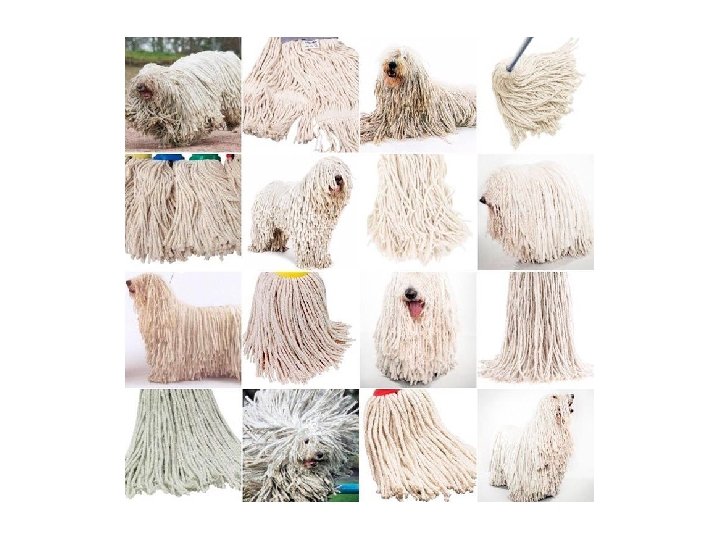
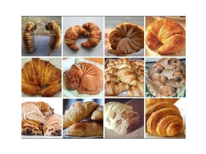
Wow false positives what class no good filtr so misclassified cool kernel
Stochastic Gradient Descent • “Epoch“
Stochastic Gradient Descent Loss will not always decrease (locally) as training data point is random. Still converges over time. Wikipedia
Gradient descent oscillations Wikipedia
Gradient descent oscillations Slow to converge to the (local) optimum Wikipedia
Momentum •
But James… …I thought we were going to treat machine learning like a black box? I like black boxes. Deep learning is: - a black box Training data Classifier
But James… …I thought we were going to treat machine learning like a black box? I like black boxes. Deep learning is: - a black box - also a black art. http: //www. isrtv. com
But James… …I thought we were going to treat machine learning like a black box? I like black boxes. Many approaches and hyperparameters: Activation functions, learning rate, mini-batch size, momentum… Often these need tweaking, and you need to know what they do to change them intelligently.
Nailing hyperparameters + trade-offs
Lowering the learning rate = smaller steps in SGD -Less ‘ping pong’ -Takes longer to get to the optimum Wikipedia
Flat regions in energy landscape
Problem of fitting • Too many parameters = overfitting • Not enough parameters = underfitting • More data = less chance to overfit • How do we know what is required?
Regularization • Attempt to guide solution to not overfit • But still give freedom with many parameters
Data fitting problem [Nielson]
Which is better? Which is better a priori? 9 th order polynomial 1 st order polynomial [Nielson]
Regularization • Attempt to guide solution to not overfit • But still give freedom with many parameters • Idea: Penalize the use of parameters to prefer small weights.
Regularization: • [Nielson]
Both can describe the data… • …but one is simpler. • Occam’s razor: “Among competing hypotheses, the one with the fewest assumptions should be selected” For us: Large weights cause large changes in behaviour in response to small changes in the input. Simpler models (or smaller changes) are more robust to noise.
Regularization • Normal cross-entropy loss (binary classes) Regularization term [Nielson]
Regularization: Dropout Our networks typically start with random weights. Every time we train = slightly different outcome. • Why random weights? • If weights are all equal, response across filters will be equivalent. • Network doesn’t train. [Nielson]
Regularization Our networks typically start with random weights. Every time we train = slightly different outcome. • Why not train 5 different networks with random starts and vote on their outcome? • Works fine! • Helps generalization because error due to overfitting is averaged; reduces variance.
Regularization: Dropout [Nielson]
Regularization: Dropout At each mini-batch: - Randomly select a subset of neurons. - Ignore them. On test: half weights outgoing to compensate for training on half neurons. Effect: - Neurons become less dependent on output of connected neurons. - Forces network to learn more robust features that are useful to more subsets of neurons. - Like averaging over many different trained networks with different random initializations. - Except cheaper to train. [Nielson]
Many forms of ‘regularization’ • Adding more data is a kind of regularization • Pooling is a kind of regularization • Data augmentation is a kind of regularization