The Convolution Integral Convolution operation given symbol y

The Convolution Integral • Convolution operation given symbol ‘*’ “y” equals “x” convolved with “h”

The Convolution Integral • The time domain output of an LTI system is equal to the convolution of the impulse response of the system with the input signal • Much simpler relationship between frequency domain input and output • First look at graphical interpretation of convolution integral

Graphical Interpretation of Convolution Integral • To correctly understand convolution it is often easier to think graphically h(t) t
 h(t) t Take impulse response and reverse it")
Graphical Interpretation of Convolution Integral h(-t) h(t) t Take impulse response and reverse it in time t
 h(t-t) t Then shift it by time t")
Graphical Interpretation of Convolution Integral h(-t) h(t-t) t Then shift it by time t t t
 x(t) t a t Overlay input function x(t)")
Graphical Interpretation of Convolution Integral h(t-t) x(t) t a t Overlay input function x(t) and integrate over times where functions overlap - in this case between a and t

Graphical Interpretation of the Convolution Integral • Convolving two functions involves – flipping or reversing one function in time – sliding this reversed or flipped function over the other and – integrating between the times when BOTH functions overlap
 x")
Example • Convolution of two gate pulses each of height 1 x 2(t) x 1(t) 0 1 t 0 2 t
 -2 Reverse function x 2(t) 0 2 t")
Example x 2(-t) -2 Reverse function x 2(t) 0 2 t
 -1 x 1(t) 0 1 t t Reverse function, slide x")
Example x 2(-t) -1 x 1(t) 0 1 t t Reverse function, slide x 2 over x 1 and evaluate integral
 x 1(t) 0 t 1 t Area of overlap is increasing")
Example x 2(t-t) x 1(t) 0 t 1 t Area of overlap is increasing linearly
 x 1(t) 0 t-2 t 1 t Area of overlap constant")
Example x 2(t-t) x 1(t) 0 t-2 t 1 t Area of overlap constant
 x 2(t-t) 0 1 t t t-2 Area declining linearly width")
Example x 1(t) x 2(t-t) 0 1 t t t-2 Area declining linearly width of shaded area = 1 -(t-2)=3 -t
 x 2(t-t) 0 t 1 t After time t=3 the convolution")
Example x 1(t) x 2(t-t) 0 t 1 t After time t=3 the convolution integral is zero
*x 2(t) 0 1 2 3 t")
Example x 1(t)*x 2(t) 0 1 2 3 t
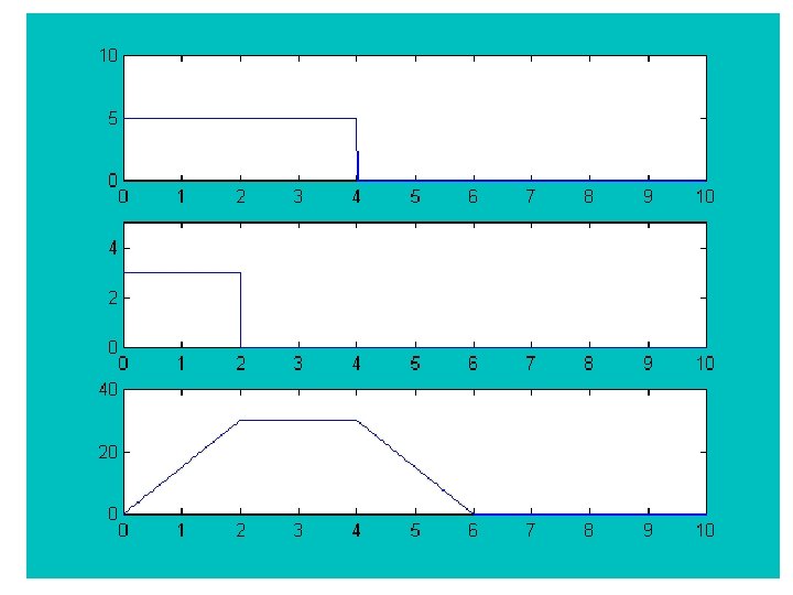
&(t<=4)); subplot(3, 1, 1), plot(t, x) axis([0")
tint=0; tfinal=10; tstep=. 01; t=tint: tstep: tfinal; x=5*((t>=0)&(t<=4)); subplot(3, 1, 1), plot(t, x) axis([0 10]) h=3*((t>=0)&(t<=2)); subplot(3, 1, 2), plot(t, h) axis([0 10]) axis([0 10 0 5]) t 2=2*tint: tstep: 2*tfinal; y=conv(x, h)*tstep; subplot(3, 1, 3), plot(t 2, y) axis([0 10 0 40])
 x 2(t) 1. 0 0")
Example 2 • Convolve the following functions x 1(t) x 2(t) 1. 0 0 1 t
 -1 Reversal 0 1 t")
Example 2 x 2(-t) -1 Reversal 0 1 t
 -1 0 t Shift reversed function 1 t")
Example 2 x 2(t-t) -1 0 t Shift reversed function 1 t
 -1 x 1(t) 0 t 1 t Overlay shift reversed")
Example 2 x 2(t-t) -1 x 1(t) 0 t 1 t Overlay shift reversed function onto other function and integrate overlapping section
 x 2(t-t) -1 0 1 t t-1 t Overlay shift")
Example 2 x 1(t) x 2(t-t) -1 0 1 t t-1 t Overlay shift reversed function onto other function and integrate overlapping section
*x 2(t) 0 1 2")
Example 2 x 1(t)*x 2(t) 0 1 2

Example 3

Example 3 5 3 t 0 4
")
Example 3 5 t Reverse h(t)
 by t t")
Example 3 5 t 4 Shift the reversed h(t) by t t

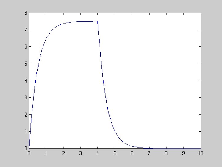
Example 3 5 t 4 Performing integral for 0<t<4 t

Example 3

Example 3 5 t 4 Performing integral for t>4 t

Example 3

Example 3

Commutativity of Convolution Operation • The actions of flipping and shifting can be applied to EITHER function
 rather than h(t)")
Example 4 • Repeat example 3 by flipping and shifting x(t) rather than h(t) 0 t

Example 4 0 t

Example 4 0 t-4 t

Example 4

Example 4 Same result as before
- Slides: 39