Perceptron ClassifierController Perceptron Learning Algorithm PLA Control theory

Perceptron Classifier/Controller Perceptron Learning Algorithm (PLA) Control theory Least Mean Square algorithm (LMS)

Perceptron Learning Algorithm (PLA)

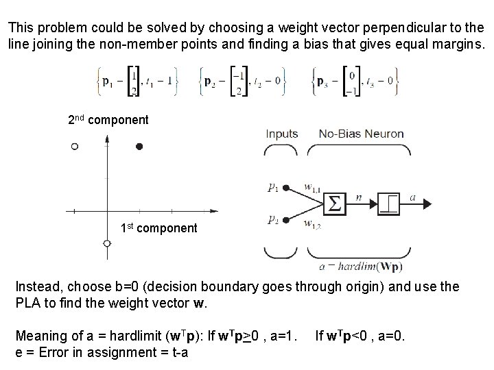
This problem could be solved by choosing a weight vector perpendicular to the line joining the non-member points and finding a bias that gives equal margins. 2 nd component 1 st component Instead, choose b=0 (decision boundary goes through origin) and use the PLA to find the weight vector w. Meaning of a = hardlimit (w. Tp): If w. Tp>0 , a=1. e = Error in assignment = t-a If w. Tp<0 , a=0.

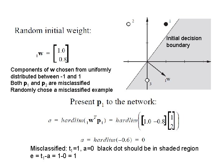
Initial decision boundary Components of w chosen from uniformly distributed between -1 and 1 Both p 1 and p 2 are misclassified Randomly chose a misclassified example Misclassified: t 1=1, a=0 black dot should be in shaded region e = t 1 -a = 1 -0 = 1

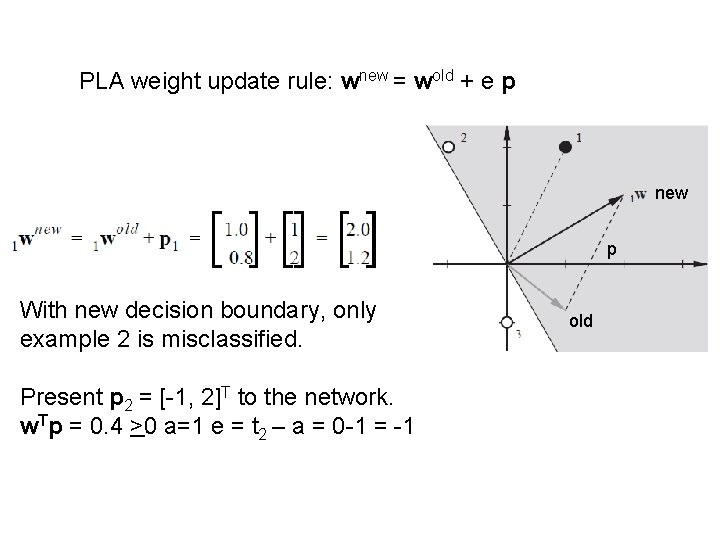
PLA weight update rule: wnew = wold + e p new p With new decision boundary, only example 2 is misclassified. Present p 2 = [-1, 2]T to the network. w. Tp = 0. 4 >0 a=1 e = t 2 – a = 0 -1 = -1 old

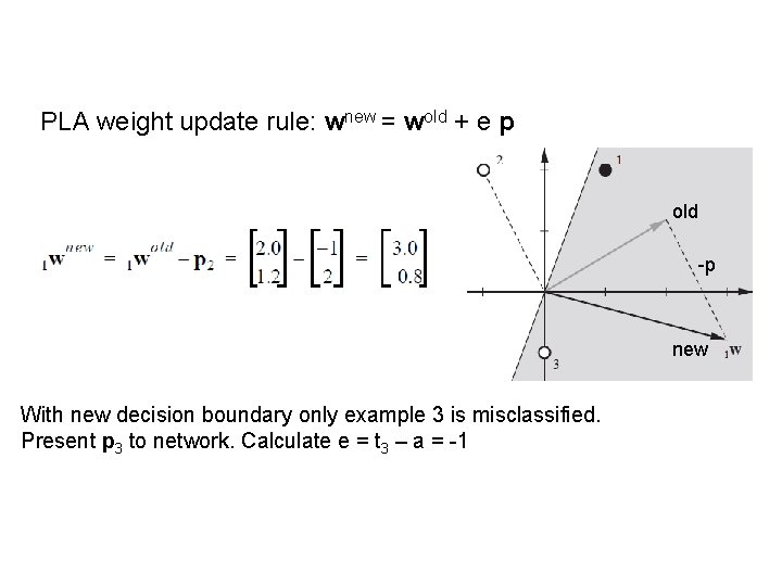
PLA weight update rule: wnew = wold + e p old -p new With new decision boundary only example 3 is misclassified. Present p 3 to network. Calculate e = t 3 – a = -1

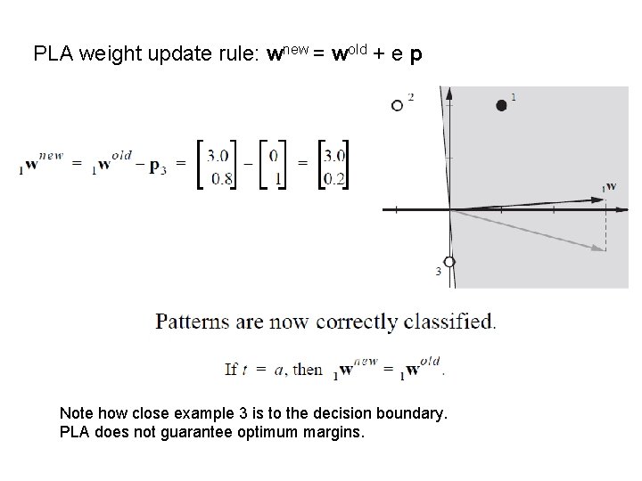
PLA weight update rule: wnew = wold + e p Note how close example 3 is to the decision boundary. PLA does not guarantee optimum margins.

Calculate class margins w. T=[3, 0. 2] ||w|| = sqrt(9+0. 04) = 3. 0067

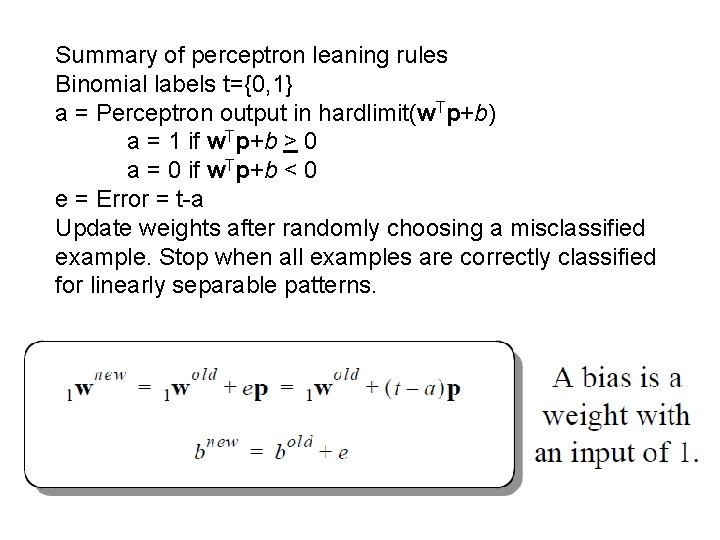
Summary of perceptron leaning rules Binomial labels t={0, 1} a = Perceptron output in hardlimit(w. Tp+b) a = 1 if w. Tp+b > 0 a = 0 if w. Tp+b < 0 e = Error = t-a Update weights after randomly choosing a misclassified example. Stop when all examples are correctly classified for linearly separable patterns.

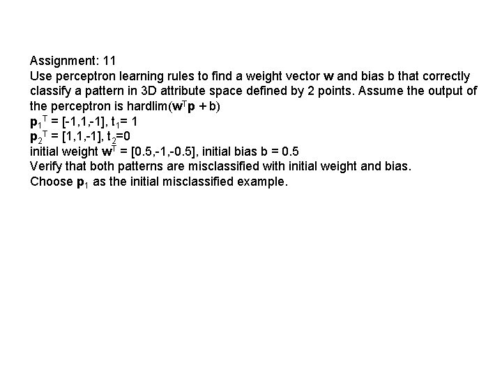
Assignment: 11 Use perceptron learning rules to find a weight vector w and bias b that correctly classify a pattern in 3 D attribute space defined by 2 points. Assume the output of the perceptron is hardlim(w. Tp + b) p 1 T = [-1, 1, -1], t 1= 1 p 2 T = [1, 1, -1], t 2=0 initial weight w. T = [0. 5, -1, -0. 5], initial bias b = 0. 5 Verify that both patterns are misclassified with initial weight and bias. Choose p 1 as the initial misclassified example.

Least Mean Square (LMS) Algorithm

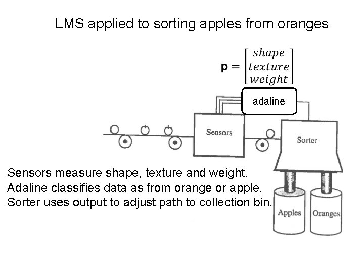
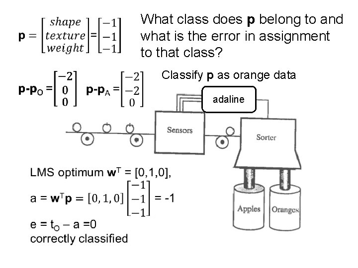
LMS applied to sorting apples from oranges A adaline Sensors measure shape, texture and weight. Adaline classifies data as from orange or apple. Sorter uses output to adjust path to collection bin.

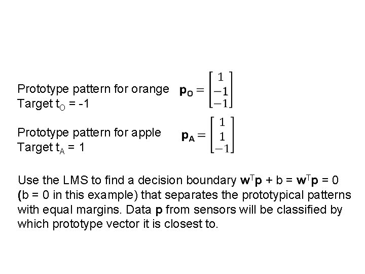
Prototype pattern for orange Target t. O = -1 Prototype pattern for apple Target t. A = 1 Use the LMS to find a decision boundary w. Tp + b = w. Tp = 0 (b = 0 in this example) that separates the prototypical patterns with equal margins. Data p from sensors will be classified by which prototype vector it is closest to.

What class does p belong to and what is the error in assignment to that class? Classify p as orange data A adaline

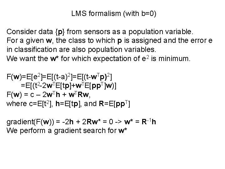
LMS formalism (with b=0) Consider data {p} from sensors as a population variable. For a given w, the class to which p is assigned and the error e in classification are also population variables. We want the w* for which expectation of e 2 is minimum. F(w)=E[e 2]=E[(t-a)2]=E[(t-w. Tp)2] =E[(t 2 -2 w. TE[tp]+w. TE[pp. T]w)] F(w) = c – 2 w. Th + w. TRw, where c=E[t 2], h=E[tp], and R=E[pp. T] gradient(F(w)) = -2 h + 2 Rw* = 0 -> w* = R-1 h We perform a gradient search for w*

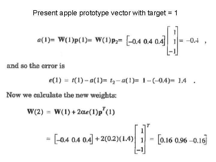
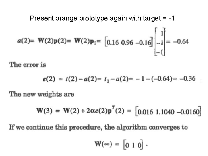
Gradient search for w* Approximate F(w)=E[e 2] by ek 2, square of error on kth iteration of the search. With no bias, ek 2(w) = (tk-w. Tpk)2 gradient(ek 2(w)) = -2 ekpk Choose a gradient-decent step size a wk+1 = wk – a gradient(ek 2(w)) wk+1 = wk + 2 aekpk Step size 0. 2 is reasonable. Initial weight vector = wi. T=[0, 0, 0]. Alternate between prototype vectors for orange and apple. a = w. Tp, e = t-a, t. O= -1, t. A = 1

Note! W(0) is a row vector = wi. T= [0, 0, 0]. Note! b = 0 in this example and t 1=t. O because p 1 is the orange prototype vector.

Present apple prototype vector with target = 1

Present orange prototype again with target = -1

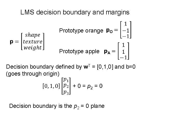
LMS decision boundary and margins Prototype orange Prototype apple Decision boundary defined by w. T = [0, 1, 0] and b=0 (goes through origin) Decision boundary is the p 2 = 0 plane

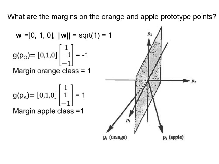
What are the margins on the orange and apple prototype points? w. T=[0, 1, 0], ||w|| = sqrt(1) = 1

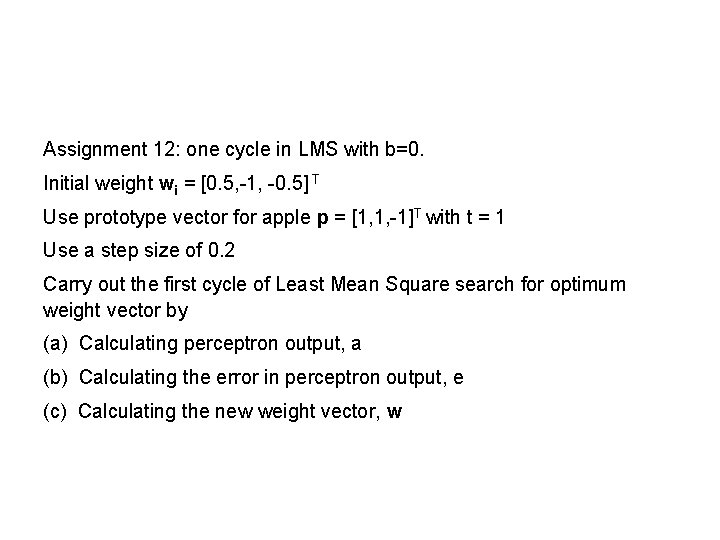
Assignment 12: one cycle in LMS with b=0. Initial weight wi = [0. 5, -1, -0. 5] T Use prototype vector for apple p = [1, 1, -1]T with t = 1 Use a step size of 0. 2 Carry out the first cycle of Least Mean Square search for optimum weight vector by (a) Calculating perceptron output, a (b) Calculating the error in perceptron output, e (c) Calculating the new weight vector, w