
Machine Learning Classifiers and Boosting Reading Ch 18
Machine Learning – Classifiers and Boosting Reading Ch 18. 6 -18. 12, 20. 1 -20. 3. 2
Outline • Different types of learning problems • Different types of learning algorithms • Supervised learning – – Decision trees Naïve Bayes Perceptrons, Multi-layer Neural Networks Boosting • Applications: learning to detect faces in images
You will be expected to know • Classifiers: – – Decision trees K-nearest neighbors Naïve Bayes Perceptrons, Support vector Machines (SVMs), Neural Networks • Decision Boundaries for various classifiers – What can they represent conveniently? What not?
Inductive learning • Let x represent the input vector of attributes – xj is the jth component of the vector x – xj is the value of the jth attribute, j = 1, …d • Let f(x) represent the value of the target variable for x – The implicit mapping from x to f(x) is unknown to us – We just have training data pairs, D = {x, f(x)} available • We want to learn a mapping from x to f, i. e. , h(x; q) is “close” to f(x) for all training data points x q are the parameters of our predictor h(. . ) • Examples: – h(x; q) = sign(w 1 x 1 + w 2 x 2+ w 3) – hk(x) = (x 1 OR x 2) AND (x 3 OR NOT(x 4))
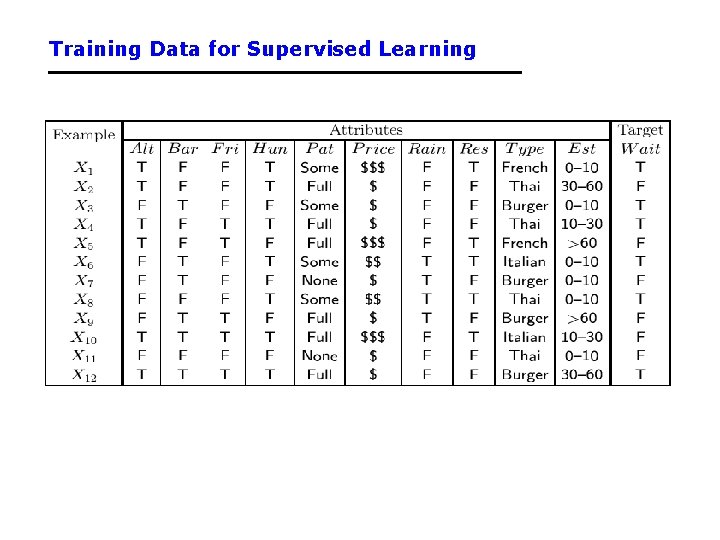
Training Data for Supervised Learning
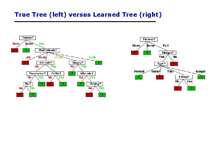
True Tree (left) versus Learned Tree (right)
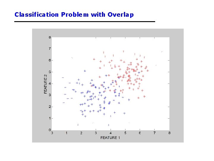
Classification Problem with Overlap
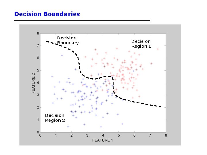
Decision Boundaries Decision Boundary Decision Region 2 Decision Region 1
Classification in Euclidean Space • A classifier is a partition of the space x into disjoint decision regions – Each region has a label attached – Regions with the same label need not be contiguous – For a new test point, find what decision region it is in, and predict the corresponding label • Decision boundaries = boundaries between decision regions – The “dual representation” of decision regions • We can characterize a classifier by the equations for its decision boundaries • Learning a classifier searching for the decision boundaries that optimize our objective function
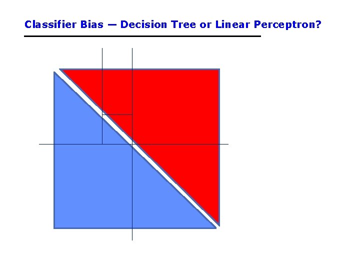
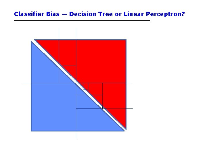
Example: Decision Trees • When applied to real-valued attributes, decision trees produce “axis-parallel” linear decision boundaries • Each internal node is a binary threshold of the form xj > t ? converts each real-valued feature into a binary one requires evaluation of N-1 possible threshold locations for N data points, for each real-valued attribute, for each internal node
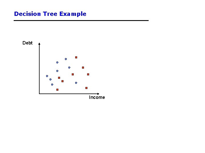
Decision Tree Example Debt Income
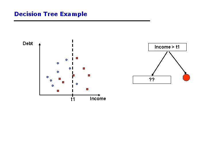
Decision Tree Example Debt Income > t 1 ? ? t 1 Income
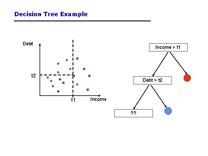
Decision Tree Example Debt Income > t 1 t 2 Debt > t 2 t 1 Income ? ?
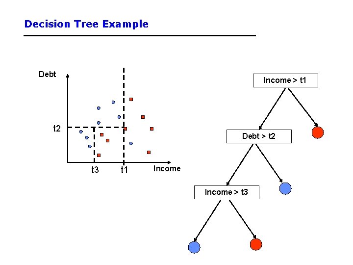
Decision Tree Example Debt Income > t 1 t 2 Debt > t 2 t 3 t 1 Income > t 3
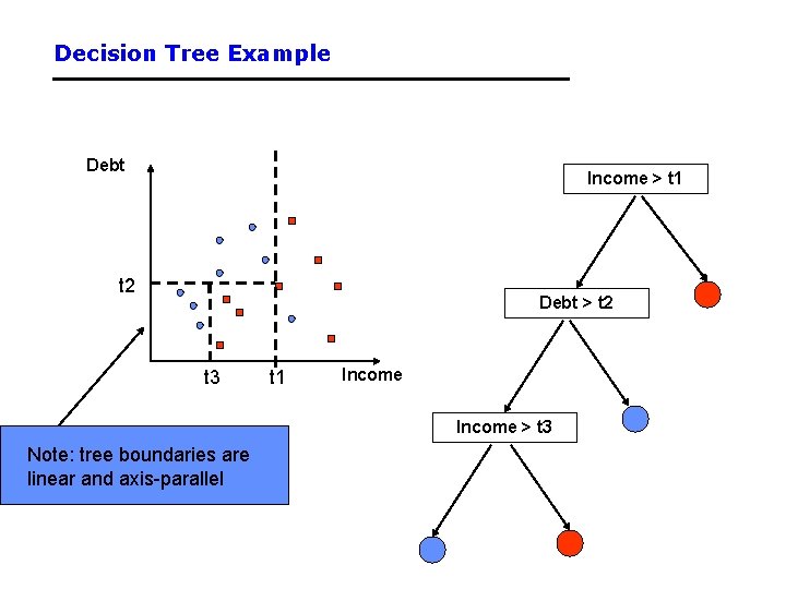
Decision Tree Example Debt Income > t 1 t 2 Debt > t 2 t 3 t 1 Income > t 3 Note: tree boundaries are linear and axis-parallel
A Simple Classifier: Minimum Distance Classifier • Training – Separate training vectors by class – Compute the mean for each class, mk, k = 1, … m • Prediction – Compute the closest mean to a test vector x’ (using Euclidean distance) – Predict the corresponding class • In the 2 -class case, the decision boundary is defined by the locus of the hyperplane that is halfway between the 2 means and is orthogonal to the line connecting them • This is a very simple-minded classifier – easy to think of cases where it will not work very well
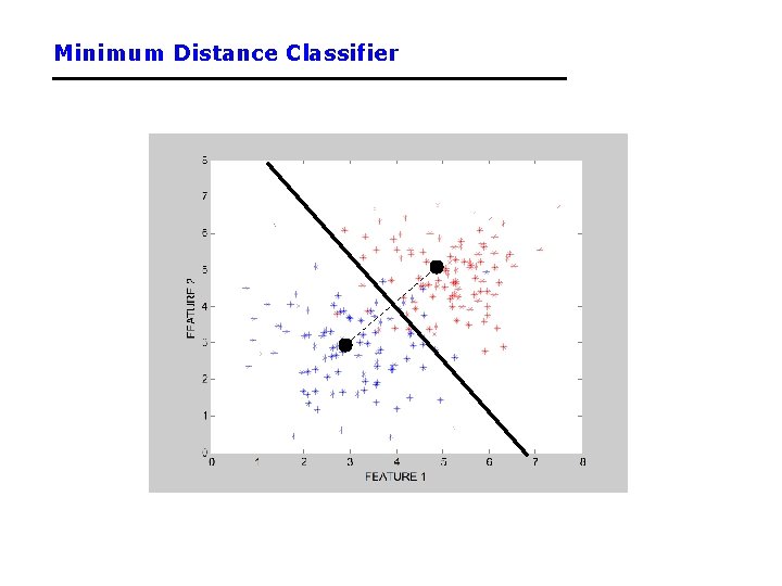
Minimum Distance Classifier
Another Example: Nearest Neighbor Classifier • The nearest-neighbor classifier – Given a test point x’, compute the distance between x’ and each input data point – Find the closest neighbor in the training data – Assign x’ the class label of this neighbor – (sort of generalizes minimum distance classifier to exemplars) • If Euclidean distance is used as the distance measure (the most common choice), the nearest neighbor classifier results in piecewise linear decision boundaries • Many extensions – e. g. , k. NN, vote based on k-nearest neighbors – k can be chosen by cross-validation
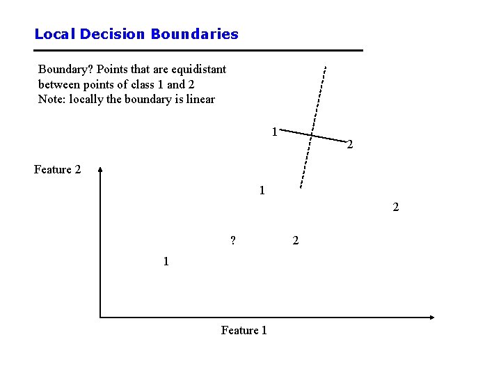
Local Decision Boundaries Boundary? Points that are equidistant between points of class 1 and 2 Note: locally the boundary is linear 1 2 Feature 2 1 2 ? 1 Feature 1 2
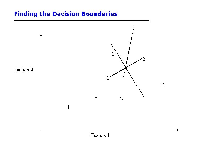
Finding the Decision Boundaries 1 2 Feature 2 1 2 ? 1 Feature 1 2
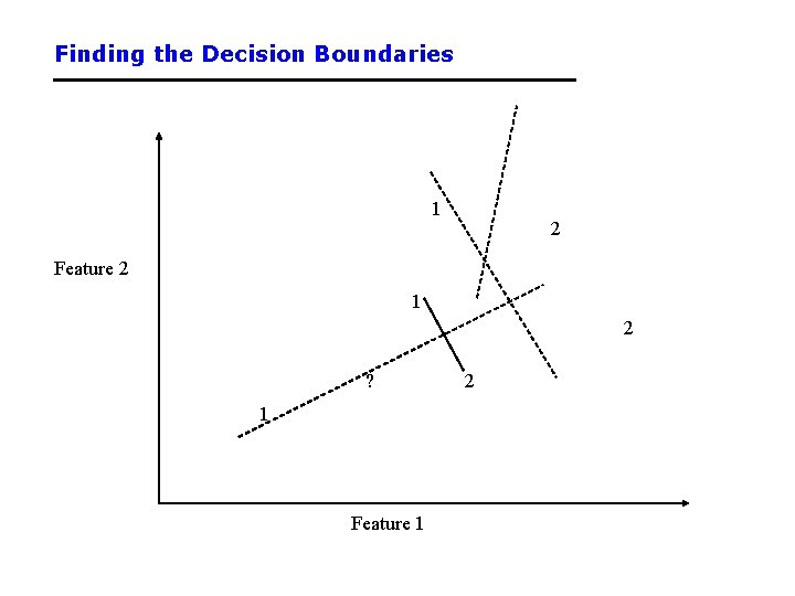
Finding the Decision Boundaries 1 2 Feature 2 1 2 ? 1 Feature 1 2
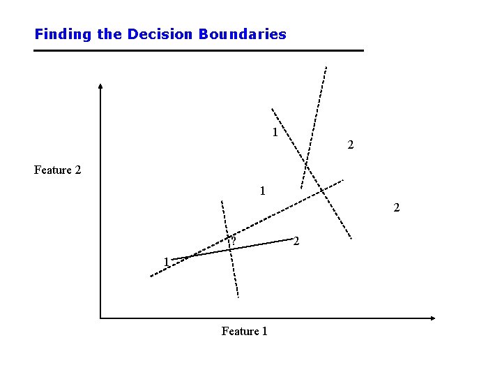
Finding the Decision Boundaries 1 2 Feature 2 1 2 ? 1 Feature 1 2
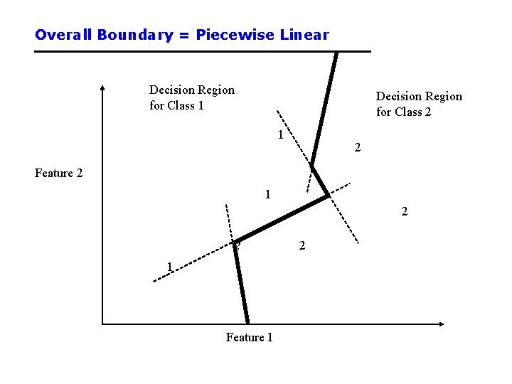
Overall Boundary = Piecewise Linear Decision Region for Class 1 Decision Region for Class 2 1 2 Feature 2 1 2 ? 1 Feature 1 2
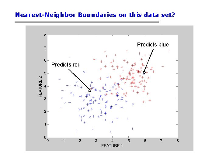
Nearest-Neighbor Boundaries on this data set? Predicts blue Predicts red
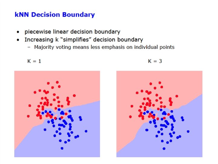
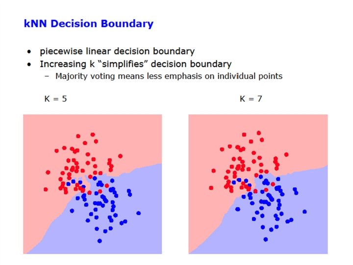
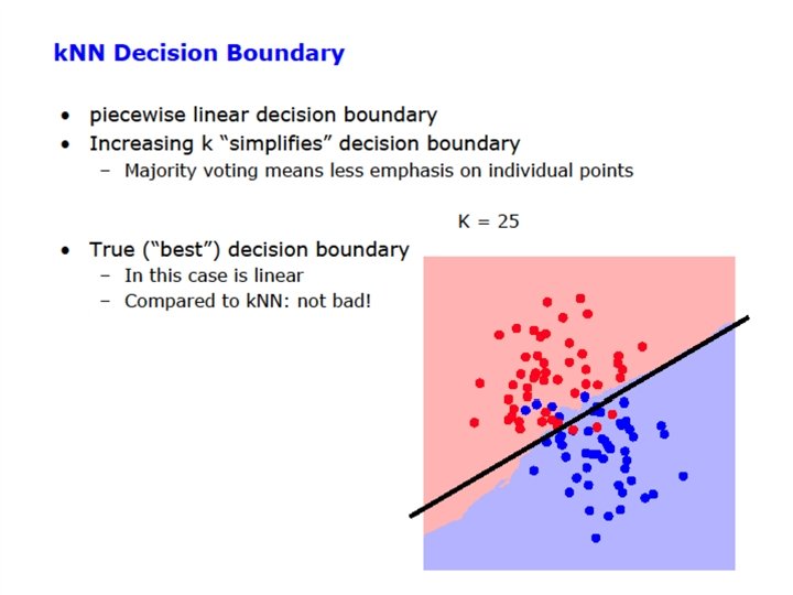
The k. NN Classifier • The k. NN classifier often works very well. • Easy to implement. • Easy choice if characteristics of your problem are unknown. • Can be sensitive to the choice of distance metric. – Often normalize feature axis values, e. g. , z-score or [0, 1] – Categorical feature axes are difficult, e. g. , Color as Red/Bue/Green • Can encounter problems with sparse training data. • Can encounter problems in very high dimensional spaces. – Most points are corners. – Most points are at the edge of the space. – Most points are neighbors of most other points.
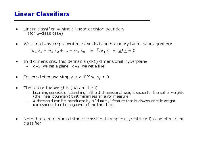
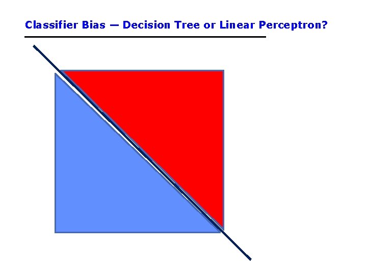
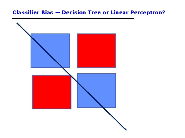
Linear Classifiers • Linear classifier single linear decision boundary (for 2 -class case) • We can always represent a linear decision boundary by a linear equation: w 1 x 1 + w 2 x 2 + … + w d xd • = wj x j In d dimensions, this defines a (d-1) dimensional hyperplane – d=3, we get a plane; d=2, we get a line wj x j > 0 • For prediction we simply see if • The wi are the weights (parameters) – – • = wt x = 0 Learning consists of searching in the d-dimensional weight space for the set of weights (the linear boundary) that minimizes an error measure A threshold can be introduced by a “dummy” feature that is always one; it weight corresponds to (the negative of) the threshold Note that a minimum distance classifier is a special (restricted) case of a linear classifier
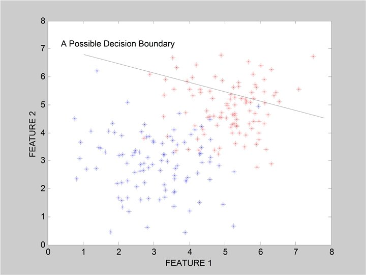
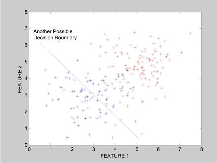
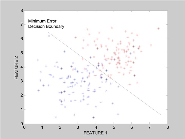
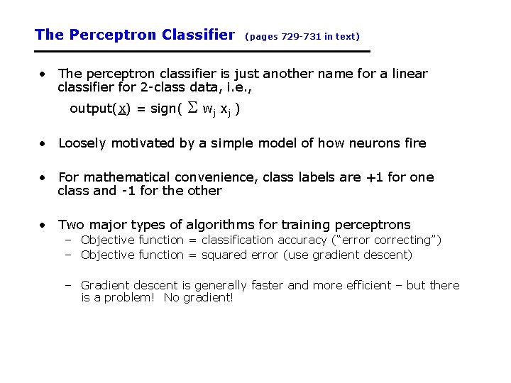
The Perceptron Classifier (pages 729 -731 in text) • The perceptron classifier is just another name for a linear classifier for 2 -class data, i. e. , output(x) = sign( wj x j ) • Loosely motivated by a simple model of how neurons fire • For mathematical convenience, class labels are +1 for one class and -1 for the other • Two major types of algorithms for training perceptrons – Objective function = classification accuracy (“error correcting”) – Objective function = squared error (use gradient descent) – Gradient descent is generally faster and more efficient – but there is a problem! No gradient!
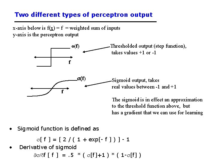
Two different types of perceptron output x-axis below is f(x) = f = weighted sum of inputs y-axis is the perceptron output o(f) Thresholded output (step function), takes values +1 or -1 f s(f) f Sigmoid output, takes real values between -1 and +1 The sigmoid is in effect an approximation to the threshold function above, but has a gradient that we can use for learning • Sigmoid function is defined as • s[ f ] = [ 2 / ( 1 + exp[- f ] ) ] - 1 Derivative of sigmoid ¶s/df [ f ] =. 5 * ( s[f]+1 ) * ( 1 -s[f] )
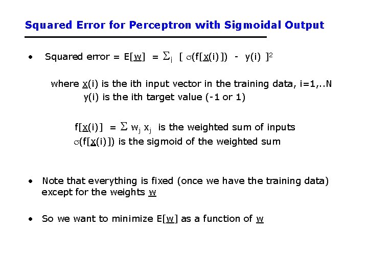
Squared Error for Perceptron with Sigmoidal Output • Squared error = E[w] = i [ s(f[x(i)]) - y(i) ]2 where x(i) is the ith input vector in the training data, i=1, . . N y(i) is the ith target value (-1 or 1) f[x(i)] = wj x j is the weighted sum of inputs s(f[x(i)]) is the sigmoid of the weighted sum • Note that everything is fixed (once we have the training data) except for the weights w • So we want to minimize E[w] as a function of w
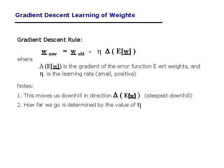
Gradient Descent Learning of Weights Gradient Descent Rule: where w new = w old - h D ( E[w] ) D (E[w]) is the gradient of the error function E wrt weights, and h is the learning rate (small, positive) Notes: D ( E[w] ) 2. How far we go is determined by the value of h 1. This moves us downhill in direction (steepest downhill)
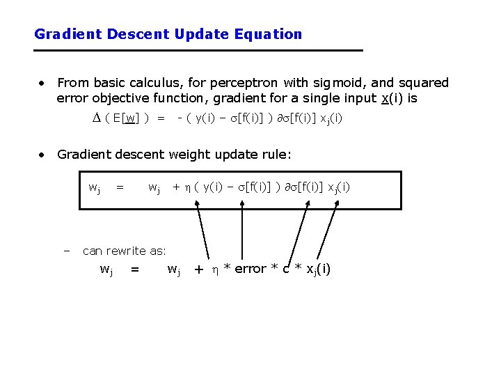
Gradient Descent Update Equation • From basic calculus, for perceptron with sigmoid, and squared error objective function, gradient for a single input x(i) is D ( E[w] ) = - ( y(i) – s[f(i)] ) ¶s[f(i)] xj(i) • Gradient descent weight update rule: wj – = wj + h ( y(i) – s[f(i)] ) ¶s[f(i)] xj(i) can rewrite as: wj = wj + h * error * c * xj(i)
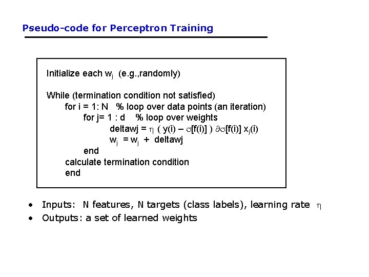
Pseudo-code for Perceptron Training Initialize each wj (e. g. , randomly) While (termination condition not satisfied) for i = 1: N % loop over data points (an iteration) for j= 1 : d % loop over weights deltawj = h ( y(i) – s[f(i)] ) ¶s[f(i)] xj(i) wj = wj + deltawj end calculate termination condition end • Inputs: N features, N targets (class labels), learning rate h • Outputs: a set of learned weights
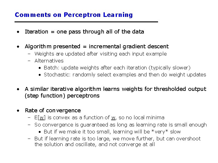
Comments on Perceptron Learning • Iteration = one pass through all of the data • Algorithm presented = incremental gradient descent – Weights are updated after visiting each input example – Alternatives • Batch: update weights after each iteration (typically slower) • Stochastic: randomly select examples and then do weight updates • A similar iterative algorithm learns weights for thresholded output (step function) perceptrons • Rate of convergence – E[w] is convex as a function of w, so no local minima – So convergence is guaranteed as long as learning rate is small enough • But if we make it too small, learning will be *very* slow – But if learning rate is too large, we move further, but can overshoot the solution and oscillate, and not converge at all
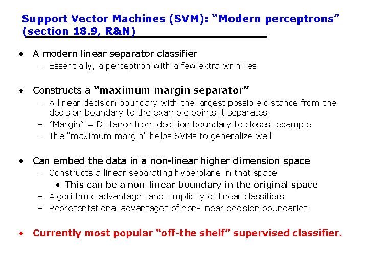
Support Vector Machines (SVM): “Modern perceptrons” (section 18. 9, R&N) • A modern linear separator classifier – Essentially, a perceptron with a few extra wrinkles • Constructs a “maximum margin separator” – A linear decision boundary with the largest possible distance from the decision boundary to the example points it separates – “Margin” = Distance from decision boundary to closest example – The “maximum margin” helps SVMs to generalize well • Can embed the data in a non-linear higher dimension space – Constructs a linear separating hyperplane in that space • This can be a non-linear boundary in the original space – Algorithmic advantages and simplicity of linear classifiers – Representational advantages of non-linear decision boundaries • Currently most popular “off-the shelf” supervised classifier.
Multi-Layer Perceptrons (Artificial Neural Networks) (sections 18. 7. 3 -18. 7. 4 in textbook) • What if we took K perceptrons and trained them in parallel and then took a weighted sum of their sigmoidal outputs? – This is a multi-layer neural network with a single “hidden” layer (the outputs of the first set of perceptrons) – If we train them jointly in parallel, then intuitively different perceptrons could learn different parts of the solution • They define different local decision boundaries in the input space • What if we hooked them up into a general Directed Acyclic Graph? – Can create simple “neural circuits” (but no feedback; not fully general) – Often called neural networks with hidden units • How would we train such a model? – Backpropagation algorithm = clever way to do gradient descent – Bad news: many local minima and many parameters • training is hard and slow – Good news: can learn general non-linear decision boundaries – Generated much excitement in AI in the late 1980’s and 1990’s – Techniques like boosting, support vector machines, are often preferred

Naïve Bayes Model X 1 X 2 (section 20. 2. 2 R&N 3 rd ed. ) X 3 Xn C Bayes Rule: P(C | X 1, …Xn) is proportional to P (C) Pi P(Xi | C) [note: denominator P(X 1, …Xn) is constant for all classes, may be ignored. ] Features Xi are conditionally independent given the class variable C • choose the class value ci with the highest P(ci | x 1, …, xn) • simple to implement, often works very well • e. g. , spam email classification: X’s = counts of words in emails Conditional probabilities P(Xi | C) can easily be estimated from labeled date • Problem: Need to avoid zeroes, e. g. , from limited training data • Solutions: Pseudo-counts, beta[a, b] distribution, etc.

Naïve Bayes Model (2) P(C | X 1, …Xn) = a P P(Xi | C) P (C) Probabilities P(C) and P(Xi | C) can easily be estimated from labeled data P(C = cj) ≈ #(Examples with class label cj) / #(Examples) P(Xi = xik | C = cj) ≈ #(Examples with Xi value xik and class label cj) / #(Examples with class label cj) Usually easiest to work with logs log [ P(C | X 1, …Xn) ] = log a + [ log P(Xi | C) + log P (C) ] DANGER: Suppose ZERO examples with Xi value xik and class label cj ? An unseen example with Xi value xik will NEVER predict class label cj ! Practical solutions: Pseudocounts, e. g. , add 1 to every #() , etc. Theoretical solutions: Bayesian inference, beta distribution, etc.
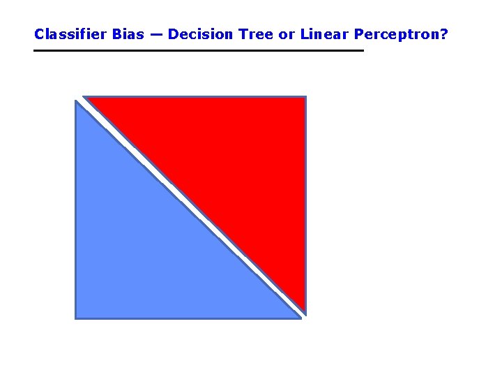
Classifier Bias — Decision Tree or Linear Perceptron?
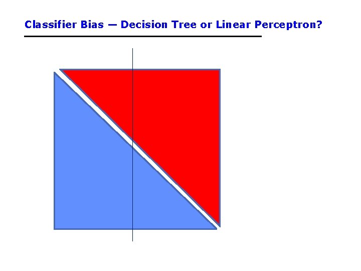
Classifier Bias — Decision Tree or Linear Perceptron?
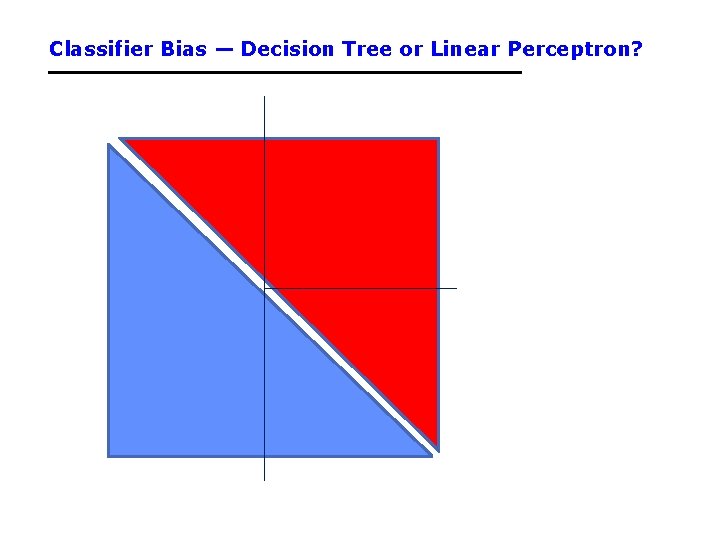
Classifier Bias — Decision Tree or Linear Perceptron?
Classifier Bias — Decision Tree or Linear Perceptron?
Classifier Bias — Decision Tree or Linear Perceptron?
Classifier Bias — Decision Tree or Linear Perceptron?
Classifier Bias — Decision Tree or Linear Perceptron?
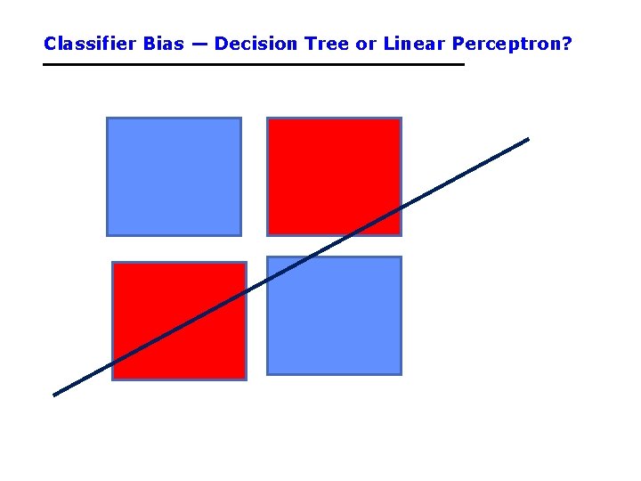
Classifier Bias — Decision Tree or Linear Perceptron?
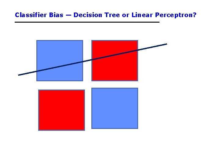
Classifier Bias — Decision Tree or Linear Perceptron?
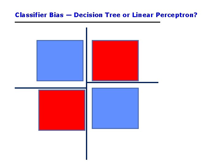
Classifier Bias — Decision Tree or Linear Perceptron?
Summary • Learning – Given a training data set, a class of models, and an error function, this is essentially a search or optimization problem • Different approaches to learning – Divide-and-conquer: decision trees – Global decision boundary learning: perceptrons – Constructing classifiers incrementally: boosting • Learning to recognize faces – Viola-Jones algorithm: state-of-the-art face detector, entirely learned from data, using boosting+decision-stumps
- Slides: 54