Feature Learning with Neural Networks aka Deep Learning

The story so far… • Neurons show increasing specificity higher in the visual pathway

Next Step • To learn good features, we need a task!

Quick Background on Supervised Learning Slides from Jitendra Malik

The MNIST DATABASE of handwritten digits yann. lecun. com/exdb/mnist/ Yann Le. Cun & Corinna

Warm-up Example: Binary Digit Classification vs.

Learning Approach to Object Recognition • Collect Training Images – Positive: – Negative: •

In feature space, positive and negative examples are just points…

Nearest neighbor rule “transfer label of nearest example”

Two kinds of error • Training set error – We train a classifier to

Historical (? ) Anecdote • In the 1970 s, DARPA wanted to find tanks

Validation and Cross-Validation • To avoid over-fitting, we can measure error on a held-out

Different approaches to training classifiers • • • Nearest neighbor methods Neural networks Support

“neural network” model • Each neuron receives inputs from other neurons • The effect

A very simple way to recognize handwritten shapes • Consider a neural network with

How to display the weights 1 2 3 4 5 6 7 8 9

How to learn the weights 1 2 3 4 5 6 7 8 9

The learned weights 1 2 3 4 5 6 7 8 9 0 The

Why the simple learning algorithm is insufficient • A two layer network with a

Non-linear classification example: XOR/XNOR , are binary (0 or 1). x 2 x 1

Simple example: AND 1. 0 0 0 1 1 0 1 Andrew Ng

Example: OR function -10 20 20 0 0 1 1 0 1 Andrew Ng

Putting it together: -30 10 -10 20 -20 20 0 0 1 1 0

Neural Network learning its own features Layer 1 Layer 2 Layer 3 Andrew Ng

Training a neural network https: //www. youtube. com/watch? v=bxe 2 T-V 8 XRs Andrew

Convolutional Neural Networks CS 194: Computer Vision and Comp. Photo Alexei Efros, UC Berkeley,

Neural Nets: a particularly useful Black Box Convolutional Neural Network image X “Penguin” label

Classic Object Recognition Feature extractors Classifier Edges Segments Texture Parts “Penguin” Colors image X

Classic Object Recognition Learned Feature extractors Classifier Edges Segments Texture Parts “Penguin” Colors image

Learning Features Learned Feature extractors Edges Texture Colors image X label Y

Neural Network: algorithm + feature + data! Learned “Penguin” image X label Y Slide

Vanilla (fully-connected) Neural Networks

Fully Connected Layer Example: 200 x 200 image 40 K hidden units ~2 B

Locally Connected Layer Example: 200 x 200 image 40 K hidden units Filter size:

Locally Connected Layer STATIONARITY? Statistics is similar at different locations Example: 200 x 200

Convolutional Layer Share the same parameters across different locations (assuming input is stationary): Convolutions

Convolutional Layer Learn multiple filters. E. g. : 200 x 200 image 100 Filters

before: input layer output layer hidden layer now: Fei-Fei Li & Andrej Karpathy Lecture

Convolution Layer 32 x 3 image 32 height 32 width 3 depth Fei-Fei Li

Convolution Layer 32 x 3 image 5 x 5 x 3 filter 32 Convolve

Convolution Layer Filters always extend the full depth of the input volume 32 x

Convolution Layer 32 32 32 x 3 image 5 x 5 x 3 filter

Convolution Layer 32 activation map 32 x 3 image 5 x 5 x 3

Convolution Layer 32 consider a second, green filter activation maps 32 x 3 image

For example, if we had 6 5 x 5 filters, we’ll get 6 separate

Slides: 84

Download presentation

Feature Learning with Neural Networks (aka Deep Learning) CS 194: Intro to Computer Vision and Comp. Photo Alexei Efros, UC Berkeley, Fall 2020

The story so far… • Neurons show increasing specificity higher in the visual pathway • V 1 simple and complex cells are orientation-tuned • Convolution with a linear kernel followed by simple non-linearities is a good model for computation in retina, LGN and V 1, but beyond that we do not have satisfactory computational models • Good designs of visual systems are likely to be hierarchical and “mostly” feedforward

Learned filters

[ slide courtesy Yann Le. Cun 4]

Next Step • To learn good features, we need a task!

Quick Background on Supervised Learning Slides from Jitendra Malik

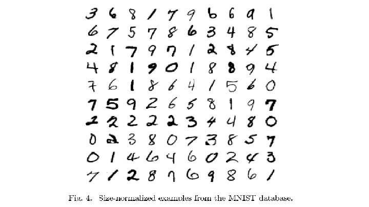
The MNIST DATABASE of handwritten digits yann. lecun. com/exdb/mnist/ Yann Le. Cun & Corinna Cortes • Has a training set of 60 K examples (6 K examples for each digit), and a test set of 10 K examples. • Each digit is a 28 x 28 pixel grey level image. The digit itself occupies the central 20 x 20 pixels, and the center of mass lies at the center of the box. • “It is a good database for people who want to try learning techniques and pattern recognition methods on real-world data while spending minimal efforts on preprocessing and formatting. ”

Warm-up Example: Binary Digit Classification vs.

Learning Approach to Object Recognition • Collect Training Images – Positive: – Negative: • Training Time – Compute feature vectors for positive and negative example images – Train a classifier • Test Time – Compute feature vector on new test image: – Evaluate classifier

Let us take an example…

In feature space, positive and negative examples are just points…

How do we classify a new point?

Nearest neighbor rule “transfer label of nearest example”

Linear classifier rule

Two kinds of error • Training set error – We train a classifier to minimize training set error. • Test set error – At run time, we will take the trained classifier and use it to classify previously unseen examples. The error on these is called test set error. • Overfitting – If the test set error is much greater than training set error

Historical (? ) Anecdote • In the 1970 s, DARPA wanted to find tanks in photographs… Positive Set Negative Set

Validation and Cross-Validation • To avoid over-fitting, we can measure error on a held-out set of training data, called the validation set. • What if we can’t spare so much data? • We could divide the data into k-folds, use k-1 of these to train and test on the remaining fold. This is cross-validation – In the limit, leave-one-out-cross-validation

Different approaches to training classifiers • • • Nearest neighbor methods Neural networks Support vector machines Randomized decision trees …

Beware of the “Half-life of Knowledge”!

“neural network” model • Each neuron receives inputs from other neurons • The effect of each input line on the neuron is controlled by a synaptic weight – The weights can be positive or negative. The synaptic weights adapt so that the whole network learns to perform useful computations – Recognizing objects, understanding language, making plans, controlling the body. You have about neurons each with about weights. • • Slide by Geoff Hinton

Source: 23 Andrej Karpathy & Fei-Fei Li

Rectified linear unit (Re. LU) 24

Rectified linear unit (Re. LU) 25

A very simple way to recognize handwritten shapes • Consider a neural network with two layers of neurons. 0 1 2 3 4 5 6 7 8 9 – neurons in the top layer represent known shapes. – neurons in the bottom layer represent pixel intensities. • A pixel gets to vote if it has ink on it. – Each inked pixel can vote for several different shapes. • The shape that gets the most votes wins. Slide by Geoff Hinton

How to display the weights 1 2 3 4 5 6 7 8 9 0 The input image Give each output unit its own “map” of the input image and display the weight coming from each pixel in the location of that pixel in the map. Use a black or white blob with the area representing the magnitude of the weight and the color representing the sign. Slide by Geoff Hinton

How to learn the weights 1 2 3 4 5 6 7 8 9 0 The image Show the network an image and increment the weights from active pixels to the correct class. Then decrement the weights from active pixels to whatever class the network guesses. Slide by Geoff Hinton

1 2 3 4 5 6 7 8 9 0 The image Slide by Geoff Hinton

The learned weights 1 2 3 4 5 6 7 8 9 0 The image Slide by Geoff Hinton

Why the simple learning algorithm is insufficient • A two layer network with a single winner in the top layer is equivalent to having a rigid template for each shape. – The winner is the template that has the biggest overlap with the ink. • The ways in which hand-written digits vary are much too complicated to be captured by simple template matches of whole shapes. Slide by Geoff Hinton

Non-linear classification example: XOR/XNOR , are binary (0 or 1). x 2 x 1 Andrew Ng

Simple example: AND 1. 0 0 0 1 1 0 1 Andrew Ng

Example: OR function -10 20 20 0 0 1 1 0 1 Andrew Ng

Negation: 0 1 Andrew Ng

Putting it together: -30 10 -10 20 -20 20 0 0 1 1 0 1 Andrew Ng

Neural Network learning its own features Layer 1 Layer 2 Layer 3 Andrew Ng

Andrew Ng

Training a neural network Andrew Ng

Training a neural network https: //www. youtube. com/watch? v=bxe 2 T-V 8 XRs Andrew Ng

Gradient descent Andrew Ng

Convolutional Neural Networks CS 194: Computer Vision and Comp. Photo Alexei Efros, UC Berkeley, Fall 2020

Neural Nets: a particularly useful Black Box Convolutional Neural Network image X “Penguin” label Y

Classic Object Recognition Feature extractors Classifier Edges Segments Texture Parts “Penguin” Colors image X label Y Slide by Philip Isola

Classic Object Recognition Learned Feature extractors Classifier Edges Segments Texture Parts “Penguin” Colors image X label Y Slide by Philip Isola

Learning Features Learned Feature extractors Edges Texture Colors image X label Y

Neural Network: algorithm + feature + data! Learned “Penguin” image X label Y Slide by Philip Isola

Vanilla (fully-connected) Neural Networks

Fully Connected Layer Example: 200 x 200 image 40 K hidden units ~2 B parameters!!! - Spatial correlation is local Waste of resources + we have not enough training samples anyway. . 56 Ranzato

Locally Connected Layer Example: 200 x 200 image 40 K hidden units Filter size: 10 x 10 4 M parameters Note: This parameterization is good when input image is registered (e. g. , face recognition). 57 Ranzato

Locally Connected Layer STATIONARITY? Statistics is similar at different locations Example: 200 x 200 image 40 K hidden units Filter size: 10 x 10 4 M parameters 58 Ranzato

Convolutional Layer Share the same parameters across different locations (assuming input is stationary): Convolutions with learned kernels 59 Ranzato

Convolutional Layer Ranzato

Convolutional Layer Learn multiple filters. E. g. : 200 x 200 image 100 Filters Filter size: 10 x 10 10 K parameters 76 Ranzato

before: input layer output layer hidden layer now: Fei-Fei Li & Andrej Karpathy Lecture 7 - 77 21 Jan 2015

Convolution Layer 32 x 3 image 32 height 32 width 3 depth Fei-Fei Li & Andrej Karpathy & Justin Johnson 7 Lecture 7 - 27 Jan 2016

Convolution Layer 32 x 3 image 5 x 5 x 3 filter 32 Convolve the filter with the image i. e. “slide over the image spatially, computing dot products” 32 3 Fei-Fei Li & Andrej Karpathy & Justin Johnson 7 Lecture 7 - 27 Jan 2016

Convolution Layer Filters always extend the full depth of the input volume 32 x 3 image 5 x 5 x 3 filter 32 Convolve the filter with the image i. e. “slide over the image spatially, computing dot products” 32 3 Fei-Fei Li & Andrej Karpathy & Justin Johnson 8 Lecture 7 - 27 Jan 2016

Convolution Layer 32 32 32 x 3 image 5 x 5 x 3 filter 1 number: the result of taking a dot product between the filter and a small 5 x 5 x 3 chunk of the image (i. e. 5*5*3 = 75 -dimensional dot product + bias) 3 Fei-Fei Li & Andrej Karpathy & Justin Johnson 8 Lecture 7 - 27 Jan 2016

Convolution Layer 32 activation map 32 x 3 image 5 x 5 x 3 filter 28 convolve (slide) over all spatial locations 28 32 3 Fei-Fei Li & Andrej Karpathy & Justin Johnson 1 8 Lecture 7 - 27 Jan 2016

Convolution Layer 32 consider a second, green filter activation maps 32 x 3 image 5 x 5 x 3 filter 28 convolve (slide) over all spatial locations 28 32 3 Fei-Fei Li & Andrej Karpathy & Justin Johnson 1 8 Lecture 7 - 27 Jan 2016

For example, if we had 6 5 x 5 filters, we’ll get 6 separate activation maps: activation maps 32 28 Convolution Layer 28 32 3 6 We stack these up to get a “new image” of size 28 x 6! Fei-Fei Li & Andrej Karpathy & Justin Johnson 8 Lecture 7 - 27 Jan 2016