Very Deep Convolutional Networks for LargeScale Image Recognition

Very Deep Convolutional Networks for Large-Scale Image Recognition By Vincent Cheong

VGG Net • Attempt to improve upon Krizhevsky et al. (2012)’s architecture. • Increasing depth while other architectural parameters are fixed.

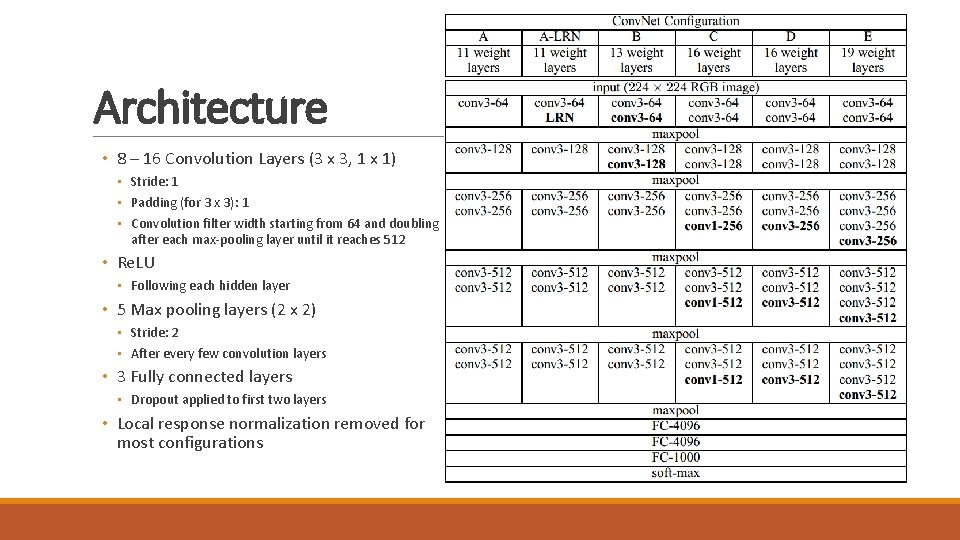
Architecture • 8 – 16 Convolution Layers (3 x 3, 1 x 1) • Stride: 1 • Padding (for 3 x 3): 1 • Convolution filter width starting from 64 and doubling after each max-pooling layer until it reaches 512 • Re. LU • Following each hidden layer • 5 Max pooling layers (2 x 2) • Stride: 2 • After every few convolution layers • 3 Fully connected layers • Dropout applied to first two layers • Local response normalization removed for most configurations

3 x 3 vs 7 x 7 Convolution Layers • A stack of three 3 x 3 conv. layers has an effective receptive field of 7 x 7. • Why three 3 x 3 layers over a single 7 x 7? • Three non-linear rectification layers instead of one • Lower number of parameters • Three 3 x 3 with C channels = 3(3 C 2) = 27 C 2 parameters • 7 x 7 = 49 C 2 parameters • 3 x 3 is the minimum size for capturing features such as left/right, up/down, and center

1 x 1 • Projection onto space of same dimensionality • Increases non-linearity without affecting receptive fields

Training • Weight initialization • Random initialization for configuration A • Layers used to initialize deeper architectures • Multinomial logistic regression utilizing mini-batch gradient descent with momentum • Image cropping • Training scale S where S is the shortest dimension of the image (Min S = 224) • Multi-scale cropping • S is randomly generated from [Smin, Smax] with Smin=256 and Smax =512 • Augmentation through scale jittering • Random horizontal flipping and RGB color shifting of crops

Testing • Multi-scale • Large difference between training and testing scales will drop performance • The smallest image side is scaled to test scale Q • Q = {S – 32, S, S+32} • Horizontal flipping of image • Dense Evaluation • • FC layers converted to convolutional layers 7 x 7, 1 x 1 Result is spatially averaged to produce a vector of class scores Applied to uncropped image • Avoids recomputation for multiple crops

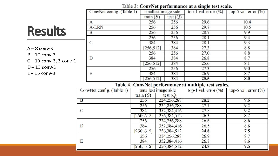
Results A – 8 conv-3 B – 10 conv-3 C – 10 conv-3, 3 conv-1 D – 13 conv-3 E – 16 conv-3

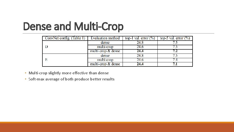
Dense and Multi-Crop • Multi-crop slightly more effective than dense • Soft-max average of both produce better results

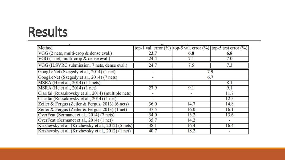
Results

Summary • LRN does not improve performance • More depth with smaller filters is better than a shallow network with large filters • Three 3 x 3 vs one 7 x 7 • Increased depth reduces classification error • Error saturates at 19 layers • Spatial context is important (3 x 3 vs 1 x 1) • Scale jittering and dense evaluation work in conjunction to improve accuracy