Step and Impulse Function Step function K t
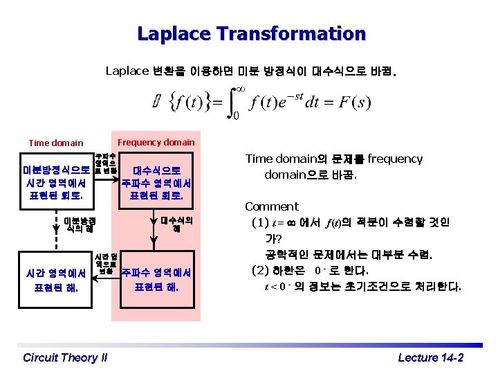


 Differentiation Integration 여기서 =0 Circuit Theory II Lecture 14 -5")
 Translation in the time domain Translation in the frequency domain Scale")
 – 초기 전압이")
 (2) (3) (4) Circuit Theory II Lecture 14 -8")
 값은 최종")
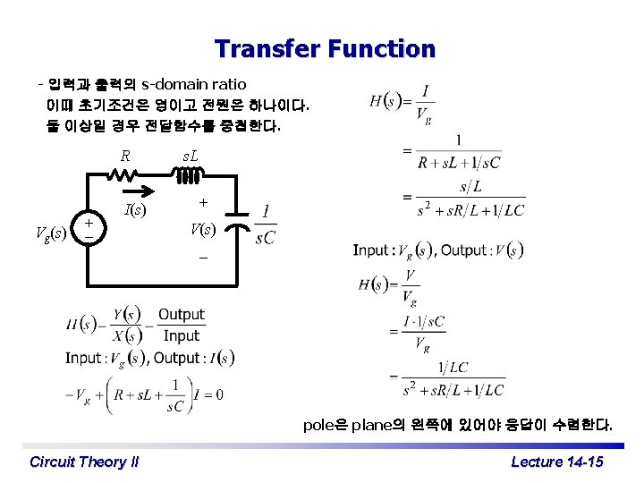
 + i v R – + V(s)")
 + v 초기전압 : V 0 Circuit")


 x(t)와 h(t)가 오직 실험 data에")

 T 1 0 (b) (d) -T 1")
 Present Future 현재: 매우 지배적 Past 미래=0 과거:")
 1. 0 vi(t- ) 0 Vo’")
- Slides: 24
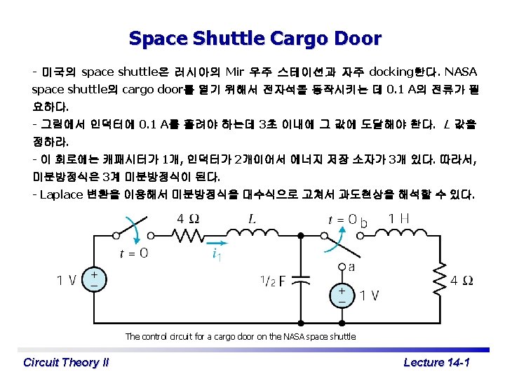
Step and Impulse Function Step function K t K 0, 면적 = 1 K (t) K (t-a) 0 Circuit Theory II a t<0 0<t K u(t-a) = 0 K u(t-a) = K t <a a<t Impulse function t a K u(t) = 0 K u(t) = K t 연속이므로 f(t) f(a) 연속이므로 f(0) = 1 Lecture 14 -3
Functional Transforms Circuit Theory II Lecture 14 -4
Operational Transforms (I) Differentiation Integration 여기서 =0 Circuit Theory II Lecture 14 -5
Operational Transforms (II) Translation in the time domain Translation in the frequency domain Scale changing Circuit Theory II Lecture 14 -6
Example + t=0 Idc R L C Laplace 변환을 하면 v(t) – 초기 전압이 영이라면 원하는 Circuit Theory II Lecture 14 -7
Inverse Transformation (1) (2) (3) (4) Circuit Theory II Lecture 14 -8
Initial-and Final-Value Theorems t = 0 또는 t = 일 때의 f(t) 값은 최종 값을 구하지 않고도 알 수 있다. Initial value Final value 1 s 이면 영. 는 상쇄되어서 Circuit Theory II 는 상쇄되어서 Lecture 14 -9
Circuit Elements in the s Domain (I) + i v R – + V(s) I(s) R – I(s) + i + 초기전류 : I 0 v L – I 0 s. L + V(s) + LI 0 – – 직렬회로 I(s) Circuit Theory II I(s) s. L 병렬회로 I(s) Lecture 14 -10
Circuit Elements in the s Domain (II) + v 초기전압 : V 0 Circuit Theory II – i I(s) + V(s) + – + V(s) I(s) CV 0 – – 직렬회로 병렬회로 Lecture 14 -11
Natural Response of an RC Circuit t=0 node a , KCL + C V 0 – R a + CV 0 V R u(t) : step function – I(s) + – Circuit Theory II R Lecture 14 -12
Step Response of a Parallel RLC Circuit 초기조건 : t=0 C R L R s. L R, L, C 값을 대입해서 부분분수 분해하고 Laplace 역변환으로 v (t) 와 i. L (t) 를 구한다. Circuit Theory II Lecture 14 -13
Transient Response of a Parallel RLC Circuit 초기조건 : t=0 C R R L s. L 정상상태 해 Circuit Theory II 과도상태 해 Lecture 14 -14
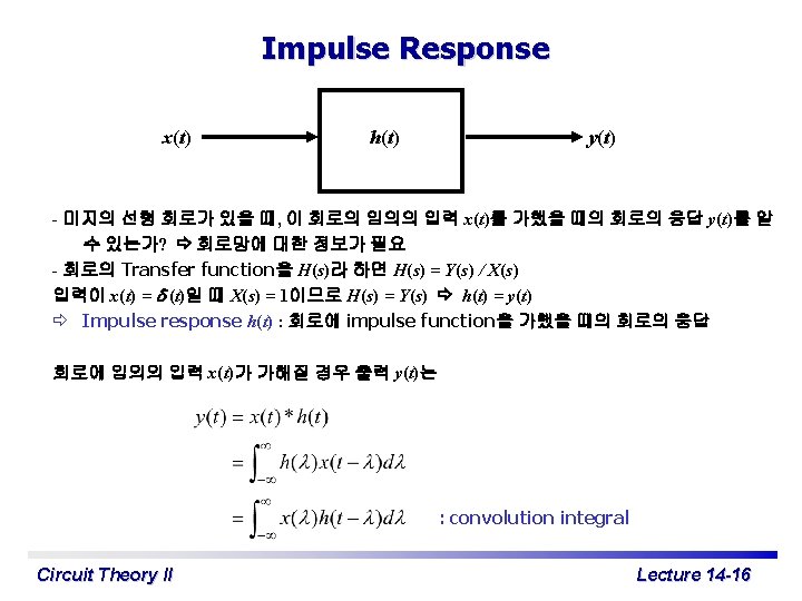
Convolution Integral 세 가지 이유에서 convolution integral을 도입. (1) x(t)와 h(t)가 오직 실험 data에 의해서만 알 수 있을 때. (2) memory와 weighting function 개념을 도입할 때. (3) Laplace 변환 함수 곱의 역 변환을 구할 때. x(t) h(t) y(t) 회로는 선형이고 time-invariant 이다. 즉, 선형이므로 superposition이 가능하고, time-invariant 이므로 input time-delay가 output에 보존되어 나타남. Input가 impulse이면 h(t) : impulse response, h(t) = y(t). Circuit Theory II Lecture 14 -17
Convolution and Laplace Transform Circuit Theory II Lecture 14 -18
Graphic Interpretation of Convolution Integral 0 (a) T 1 0 (b) (d) -T 1 MA (e) Circuit Theory II 0 t y(t)=area t-T 1 t T 2 T 1 0 (c) h(- ) (d) h( )x(t- ) 0 M x(t- ) t-T 1 x( ) A M t-T 2 0 (b) x(- ) 0 0 M T 2 M (c) -T 2 (a) x( ) M h( ) A h(t- ) y(t)=area MA (e) 0 t 0 T 1 t x( )h(t- ) Lecture 14 -19
Memory and Weighting Function h( ) Present Future 현재: 매우 지배적 Past 미래=0 과거: 덜 지배적 Perfect memory : impulse response or weighting function perfect memory h( ) No memory: h( ) 현재 과거 1. 0 Circuit Theory II Scaled replica of the input. Lecture 14 -20
Memory and Weighting Function - Example h( ) 1. 0 vi(t- ) 0 Vo’ Vi (V) 20 20 (t-10) (t-5) 0 t 5 10 vi(t- ) 현재 값이 중시 되었음. Excitation 18 16 14 12 (t-10) 0 (t-5) 5 t 10 Response 10 8 vi(t- ) 과거 값이 영향 을 미침. 6 20 4 2 0 (t-10) 5 (t-5) 10 t Circuit Theory II 0 2 4 6 8 10 12 14 Lecture 14 -21