Perceptrons and Logistic Regression Linear Classifiers Feature Vectors

Perceptrons and Logistic Regression

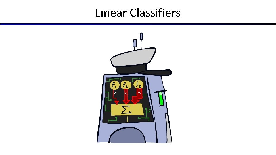
Linear Classifiers

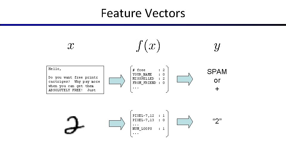
Feature Vectors Hello, Do you want free printr cartriges? Why pay more when you can get them ABSOLUTELY FREE! Just # free YOUR_NAME MISSPELLED FROM_FRIEND. . . : : 2 0 PIXEL-7, 12 PIXEL-7, 13. . . NUM_LOOPS. . . : 1 : 0 : 1 SPAM or + “ 2”

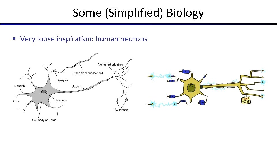
Some (Simplified) Biology § Very loose inspiration: human neurons

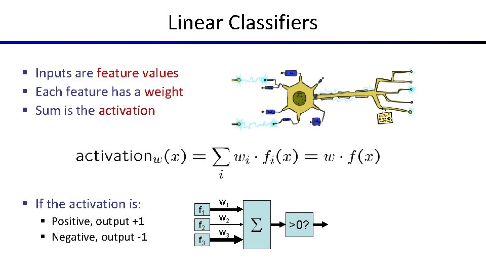
Linear Classifiers § Inputs are feature values § Each feature has a weight § Sum is the activation § If the activation is: § Positive, output +1 § Negative, output -1 f 2 f 3 w 1 w 2 w 3 >0?

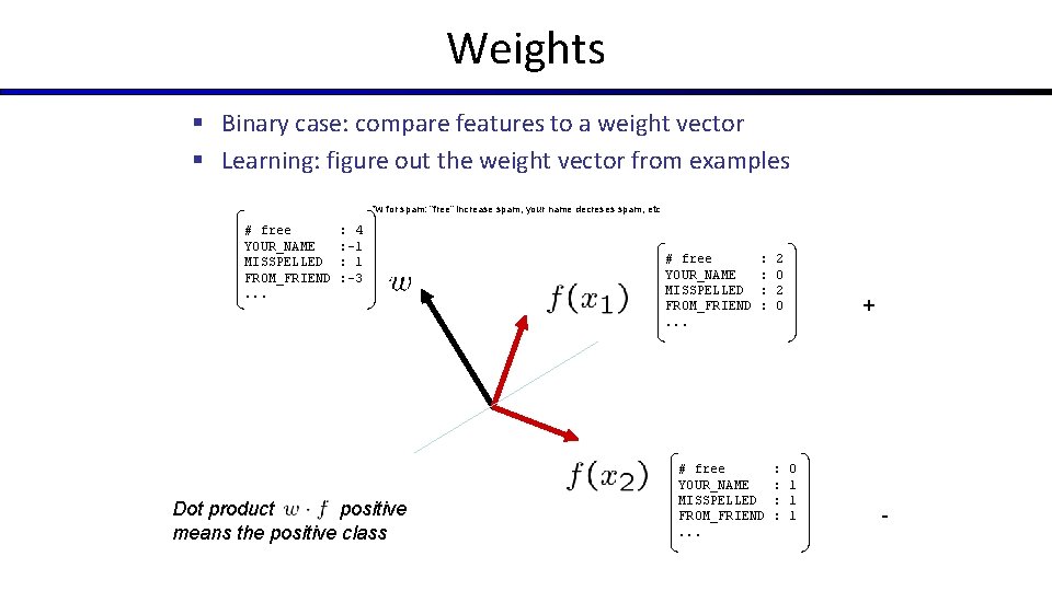
Weights § Binary case: compare features to a weight vector § Learning: figure out the weight vector from examples *w for spam: “free” increase spam, your name decreses spam, etc # free YOUR_NAME MISSPELLED FROM_FRIEND. . . : 4 : -1 : -3 Dot product positive means the positive class # free YOUR_NAME MISSPELLED FROM_FRIEND. . . : : 2 0 # free YOUR_NAME MISSPELLED FROM_FRIEND. . . : : + 0 1 1 1 -

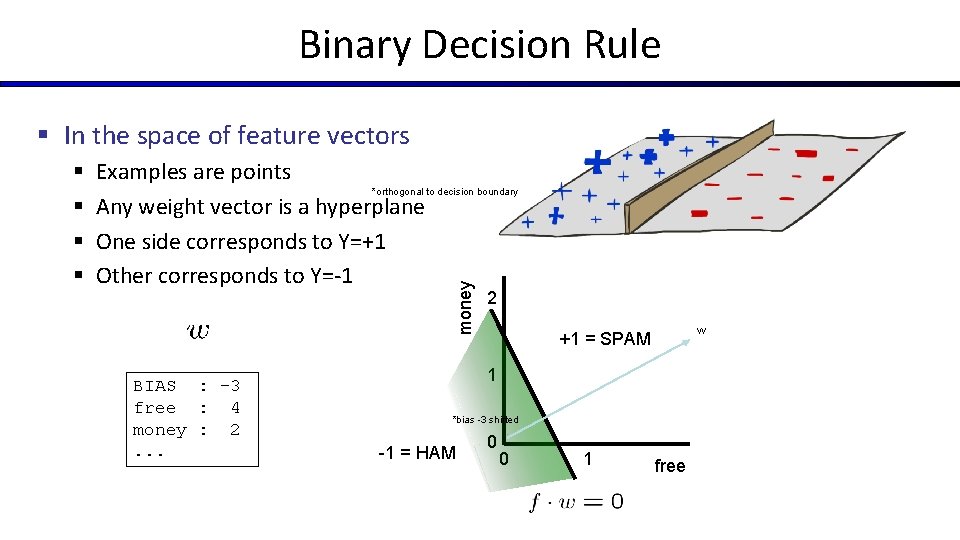
Binary Decision Rule § In the space of feature vectors Examples are points *orthogonal to decision boundary Any weight vector is a hyperplane One side corresponds to Y=+1 Other corresponds to Y=-1 money § § BIAS : -3 free : 4 money : 2. . . 2 w +1 = SPAM 1 *bias -3 shifted -1 = HAM 0 0 1 free

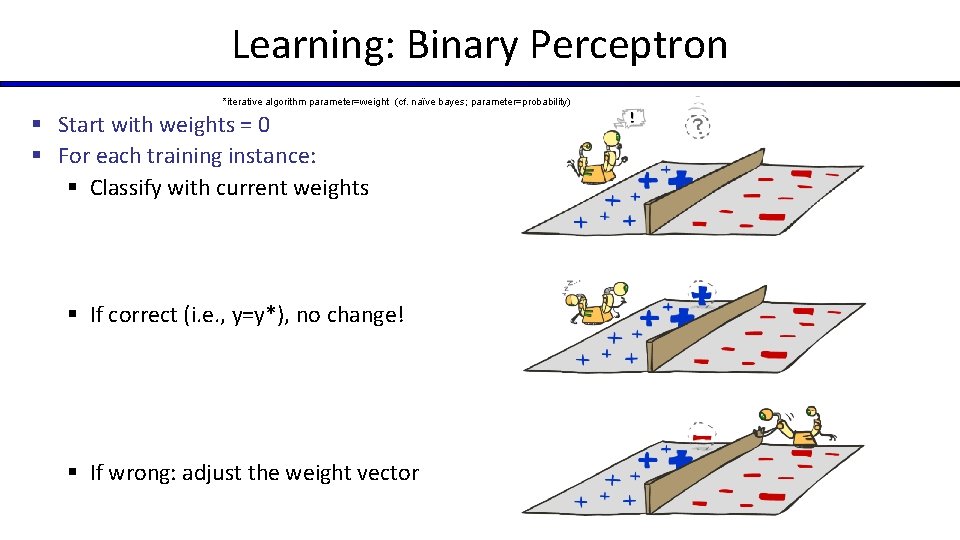
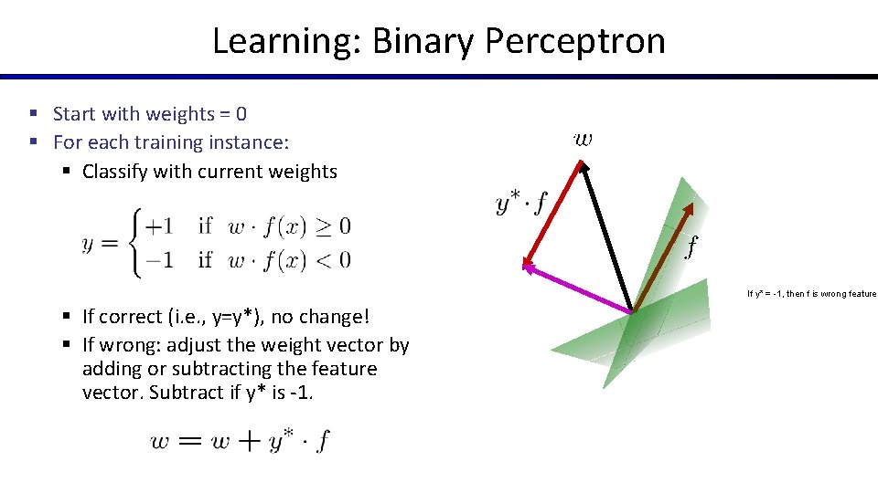
Learning: Binary Perceptron *iterative algorithm parameter=weight (cf. naïve bayes; parameter=probability) § Start with weights = 0 § For each training instance: § Classify with current weights § If correct (i. e. , y=y*), no change! § If wrong: adjust the weight vector

Learning: Binary Perceptron § Start with weights = 0 § For each training instance: § Classify with current weights If y* = -1, then f is wrong feature § If correct (i. e. , y=y*), no change! § If wrong: adjust the weight vector by adding or subtracting the feature vector. Subtract if y* is -1.

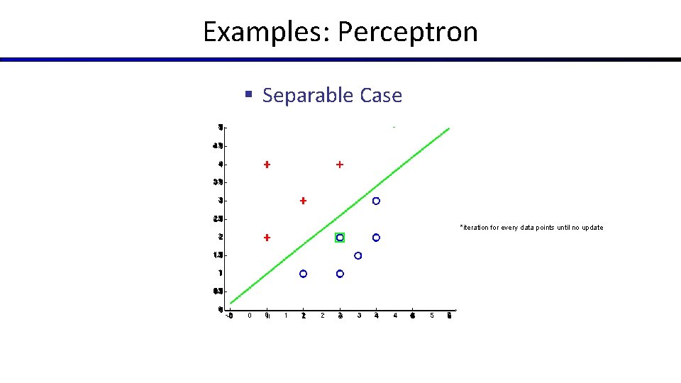
Examples: Perceptron § Separable Case *iteration for every data points until no update

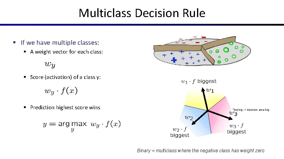
Multiclass Decision Rule § If we have multiple classes: § A weight vector for each class: § Score (activation) of a class y: § Prediction highest score wins *|w| big -> decision area big Binary = multiclass where the negative class has weight zero

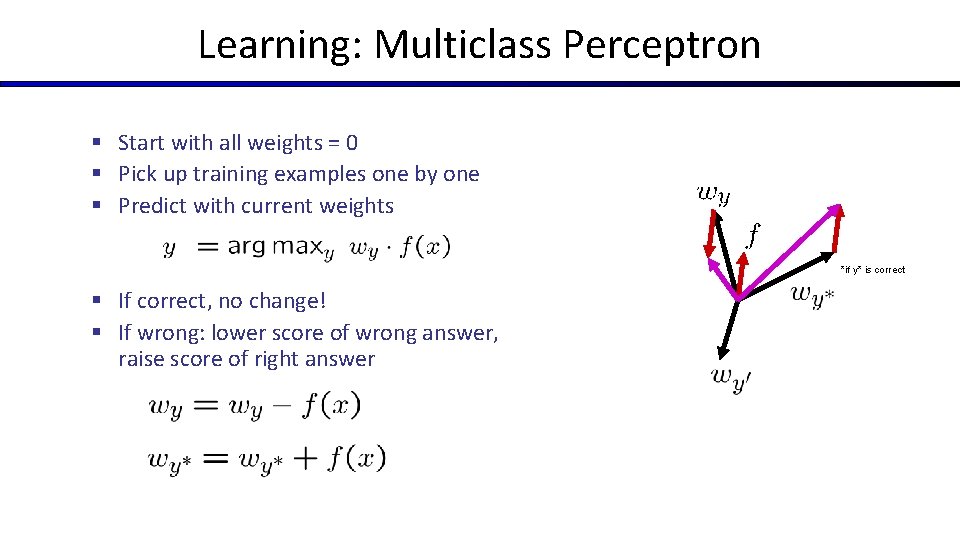
Learning: Multiclass Perceptron § Start with all weights = 0 § Pick up training examples one by one § Predict with current weights *if y* is correct § If correct, no change! § If wrong: lower score of wrong answer, raise score of right answer

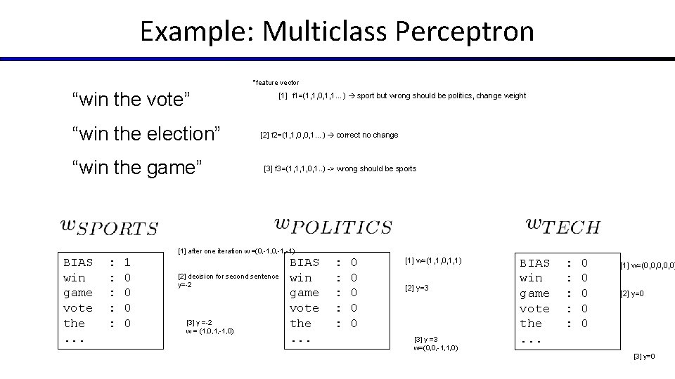
Example: Multiclass Perceptron *feature vector “win the vote” “win the election” “win the game” [1] f 1=(1, 1, 0, 1, 1…) sport but wrong should be politics, change weight [2] f 2=(1, 1, 0, 0, 1…) correct no change [3] f 3=(1, 1, 1, 0, 1. . ) -> wrong should be sports [1] after one iteration w =(0, -1, -1) BIAS win game vote the. . . : : : 1 0 0 [2] decision for second sentence y=-2 [3] y =-2 w = (1, 0, 1, -1, 0) BIAS win game vote the. . . : : : 0 0 0 [1] w=(1, 1, 0, 1, 1) [2] y=3 [3] y =3 w=(0, 0, -1, 1, 0) BIAS win game vote the. . . : : : 0 0 0 [1] w=(0, 0, 0) [2] y=0 [3] y=0

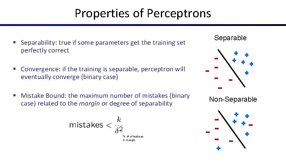
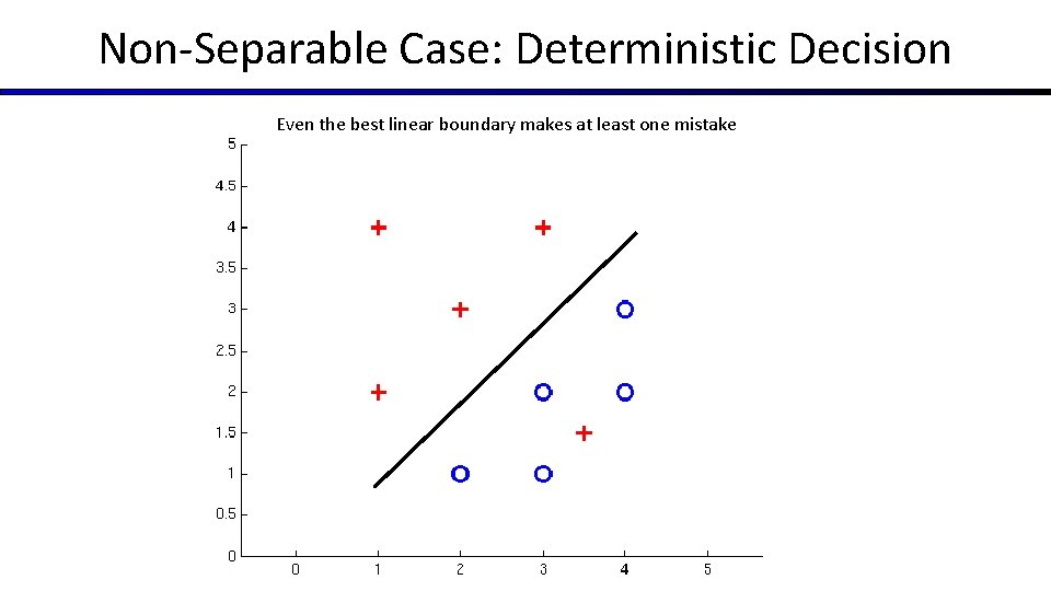
Properties of Perceptrons § Separability: true if some parameters get the training set perfectly correct Separable § Convergence: if the training is separable, perceptron will eventually converge (binary case) § Mistake Bound: the maximum number of mistakes (binary case) related to the margin or degree of separability *k: # of features d: margin Non-Separable

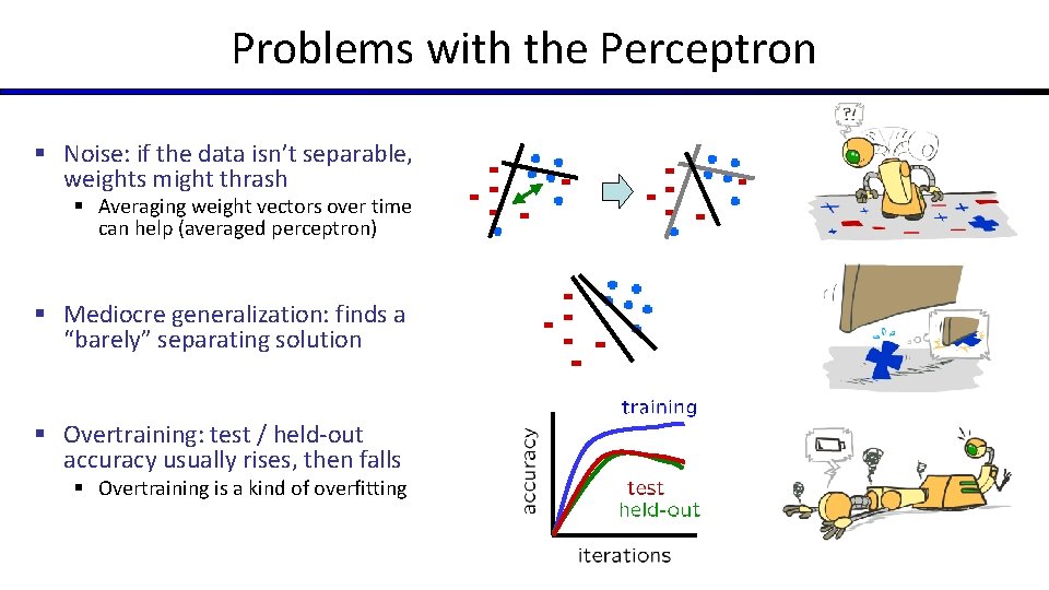
Problems with the Perceptron § Noise: if the data isn’t separable, weights might thrash § Averaging weight vectors over time can help (averaged perceptron) § Mediocre generalization: finds a “barely” separating solution § Overtraining: test / held-out accuracy usually rises, then falls § Overtraining is a kind of overfitting

Improving the Perceptron

Non-Separable Case: Deterministic Decision Even the best linear boundary makes at least one mistake

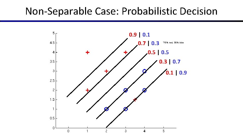
Non-Separable Case: Probabilistic Decision 0. 9 | 0. 1 0. 7 | 0. 3 0. 5 | 0. 5 *70% red, 30% blue 0. 3 | 0. 7 0. 1 | 0. 9

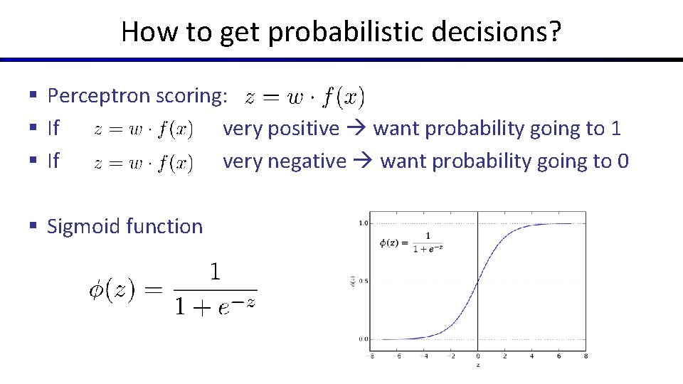
How to get probabilistic decisions? § Perceptron scoring: § If very positive want probability going to 1 § If very negative want probability going to 0 § Sigmoid function

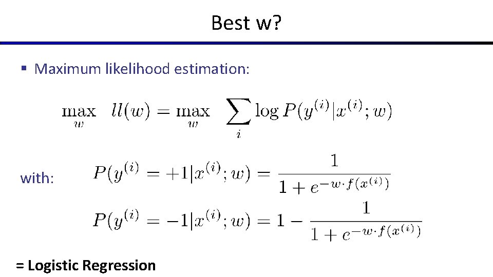
Best w? § Maximum likelihood estimation: with: = Logistic Regression

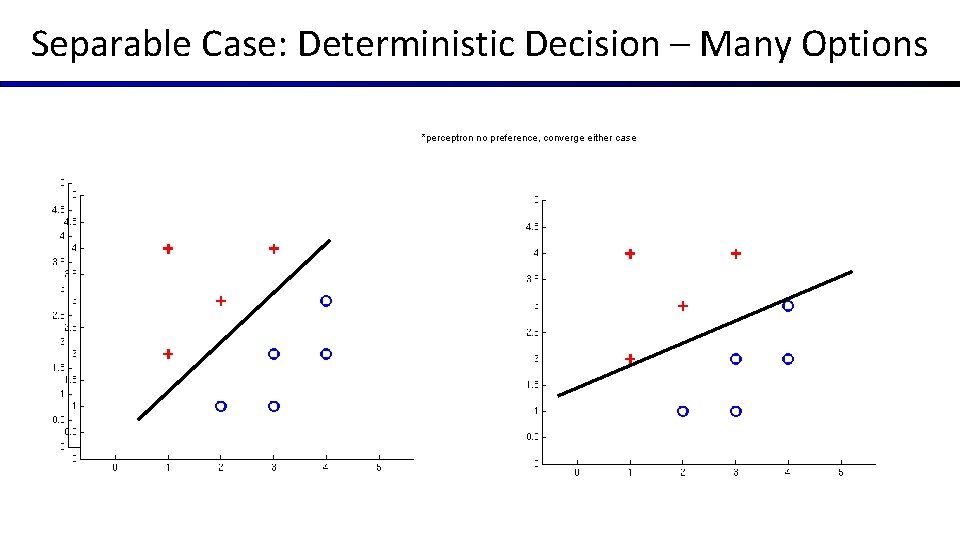
Separable Case: Deterministic Decision – Many Options *perceptron no preference, converge either case

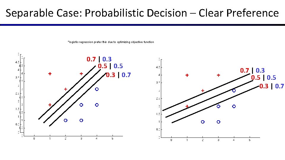
Separable Case: Probabilistic Decision – Clear Preference *logistic regression prefer this due to optimizing objective function 0. 7 | 0. 3 0. 5 | 0. 5 0. 3 | 0. 7

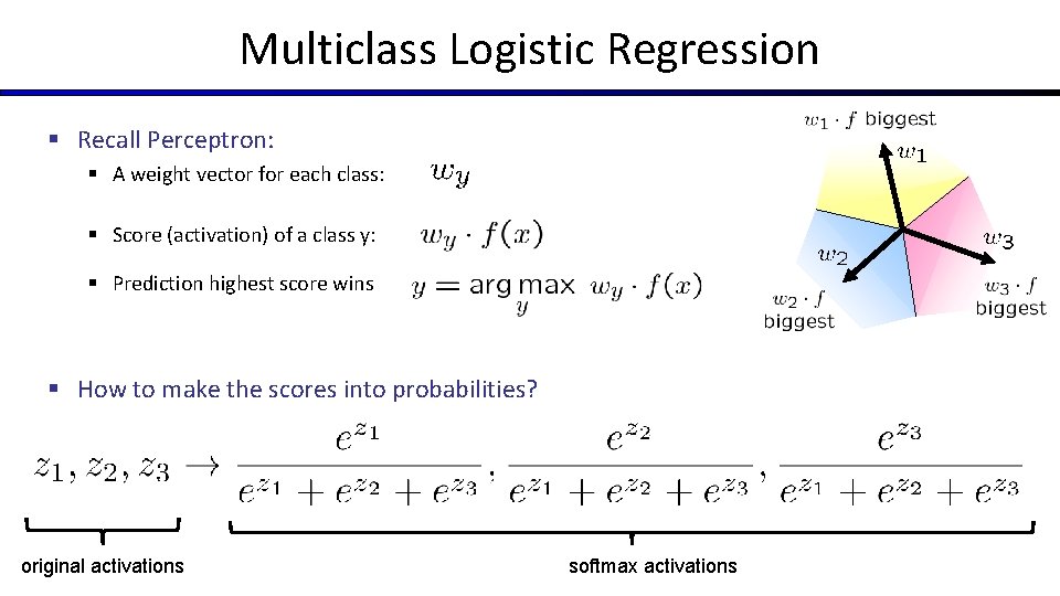
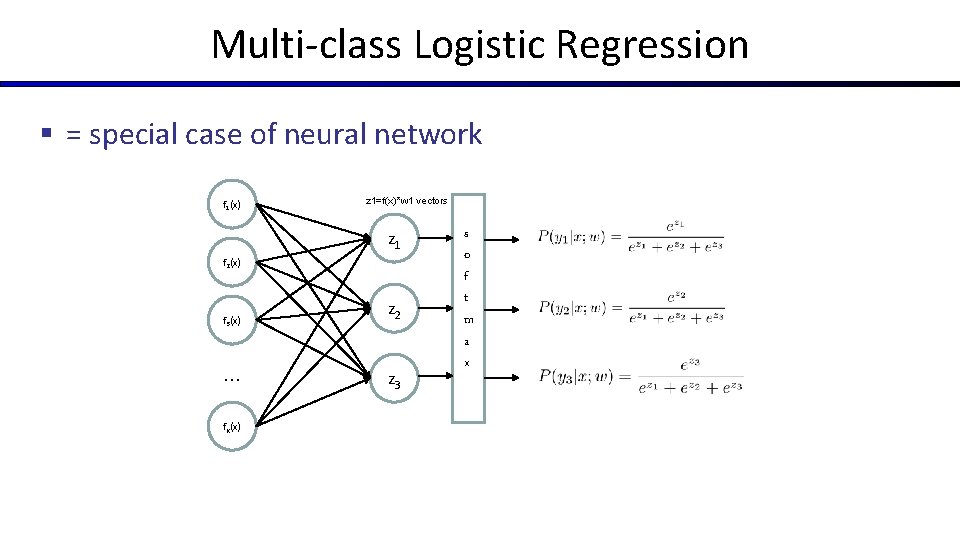
Multiclass Logistic Regression § Recall Perceptron: § A weight vector for each class: § Score (activation) of a class y: § Prediction highest score wins § How to make the scores into probabilities? original activations softmax activations

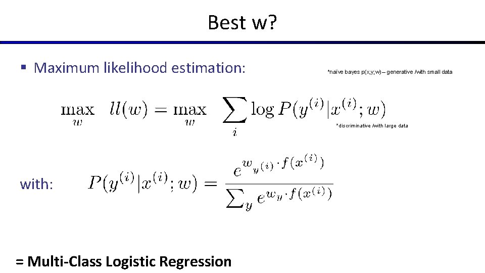
Best w? § Maximum likelihood estimation: *naïve bayes p(x, y; w) – generative /with small data *discriminative /with large data with: = Multi-Class Logistic Regression

Optimization and Neural Nets

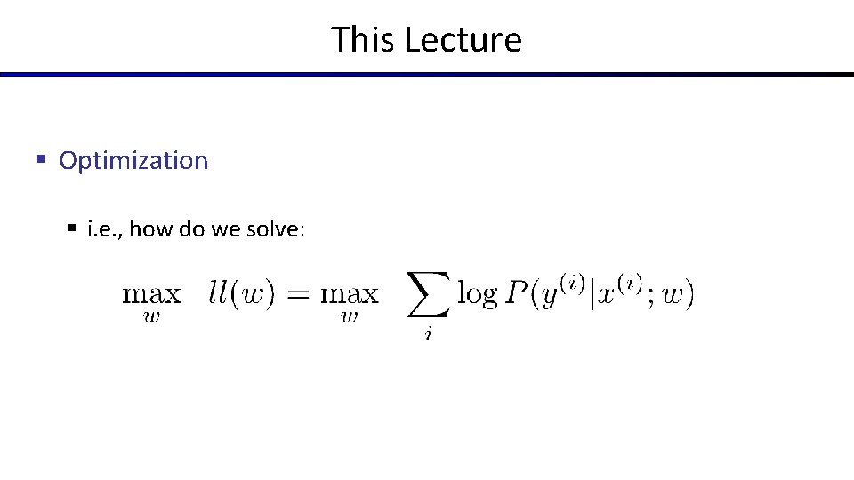
This Lecture § Optimization § i. e. , how do we solve:

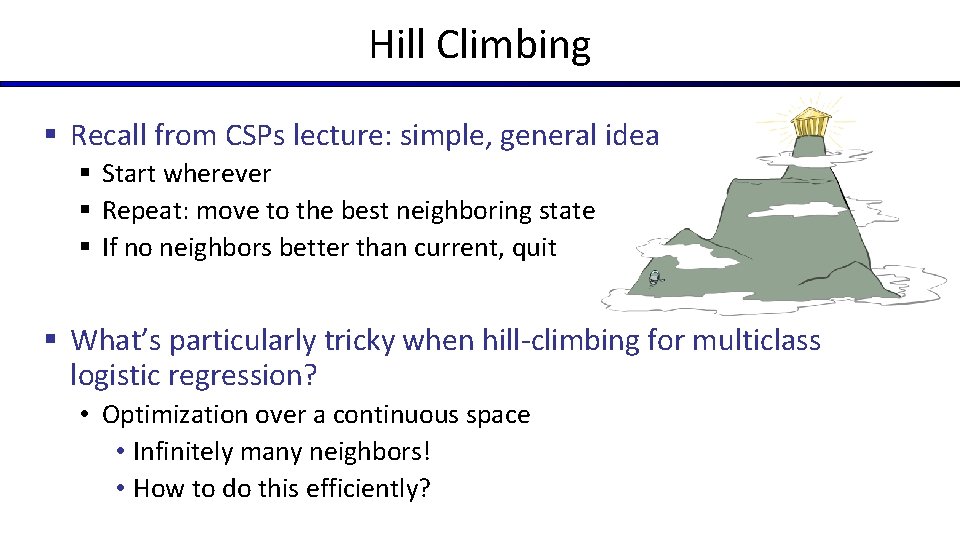
Hill Climbing § Recall from CSPs lecture: simple, general idea § Start wherever § Repeat: move to the best neighboring state § If no neighbors better than current, quit § What’s particularly tricky when hill-climbing for multiclass logistic regression? • Optimization over a continuous space • Infinitely many neighbors! • How to do this efficiently?

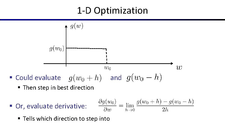
1 -D Optimization § Could evaluate § Then step in best direction § Or, evaluate derivative: § Tells which direction to step into and

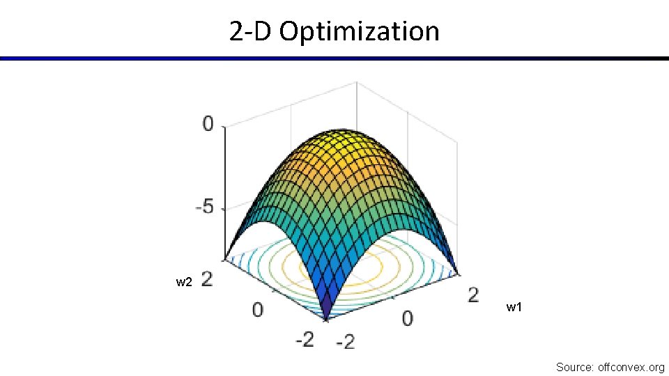
2 -D Optimization w 2 w 1 Source: offconvex. org

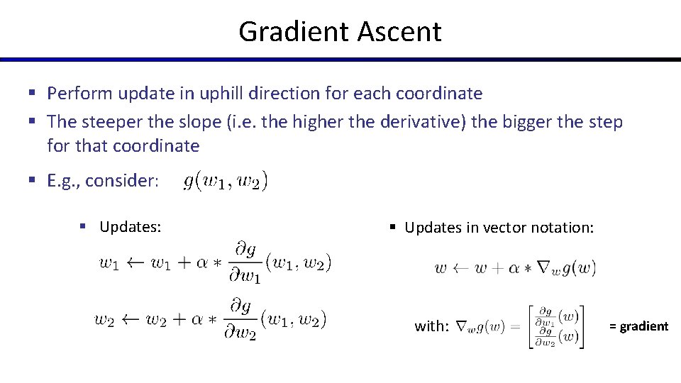
Gradient Ascent § Perform update in uphill direction for each coordinate § The steeper the slope (i. e. the higher the derivative) the bigger the step for that coordinate § E. g. , consider: § Updates: § Updates in vector notation: with: = gradient

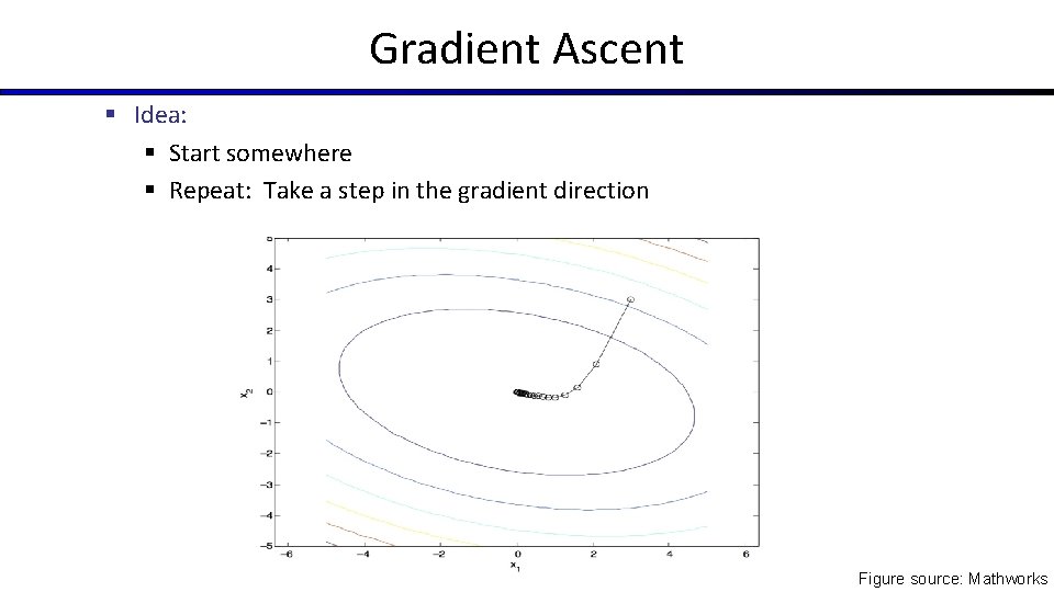
Gradient Ascent § Idea: § Start somewhere § Repeat: Take a step in the gradient direction Figure source: Mathworks

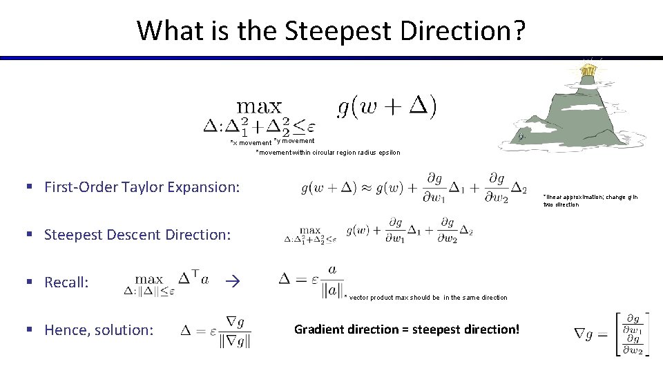
What is the Steepest Direction? *x movement *y movement *movement within circular region radius epsilon § First-Order Taylor Expansion: *linear approximation; change g in two direction § Steepest Descent Direction: § Recall: * vector product max should be in the same direction § Hence, solution: Gradient direction = steepest direction!

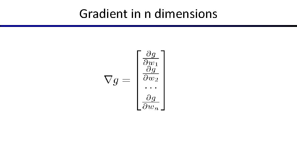
Gradient in n dimensions

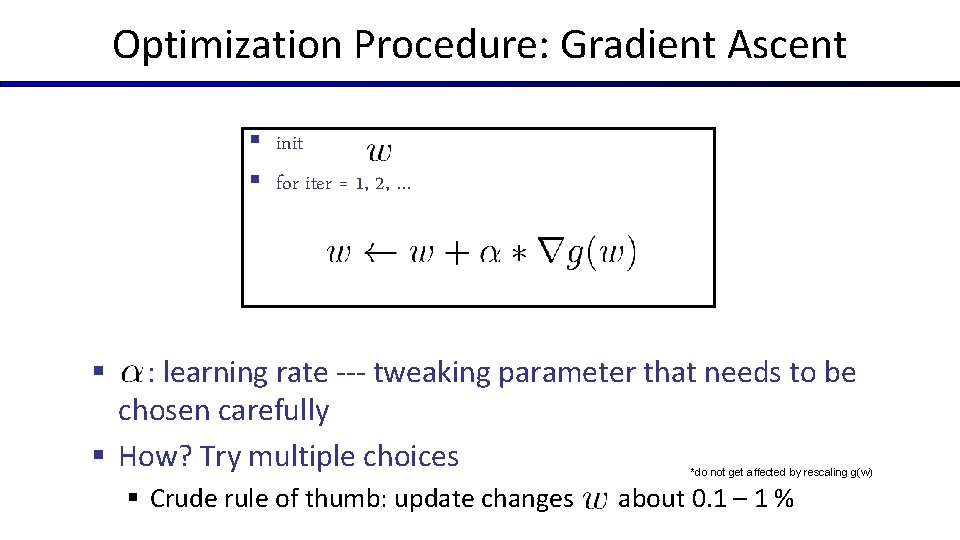
Optimization Procedure: Gradient Ascent § init § for iter = 1, 2, … : learning rate --- tweaking parameter that needs to be chosen carefully § How? Try multiple choices § *do not get affected by rescaling g(w) § Crude rule of thumb: update changes about 0. 1 – 1 %

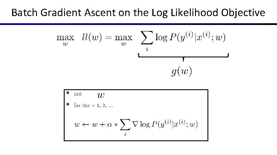
Batch Gradient Ascent on the Log Likelihood Objective § init § for iter = 1, 2, …

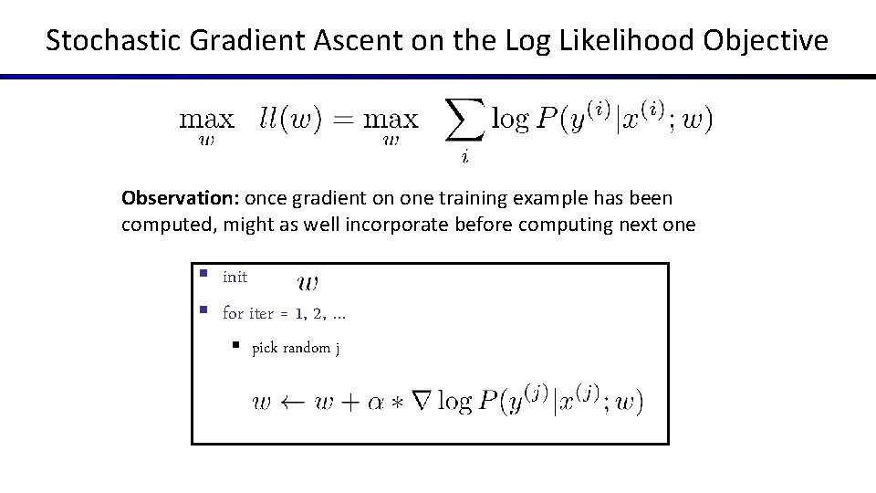
Stochastic Gradient Ascent on the Log Likelihood Objective Observation: once gradient on one training example has been computed, might as well incorporate before computing next one § init § for iter = 1, 2, … § pick random j

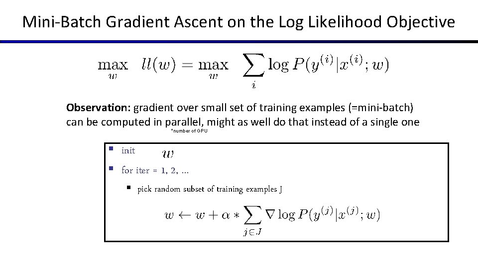
Mini-Batch Gradient Ascent on the Log Likelihood Objective Observation: gradient over small set of training examples (=mini-batch) can be computed in parallel, might as well do that instead of a single one *number of GPU § init § for iter = 1, 2, … § pick random subset of training examples J

How about computing all the derivatives? § We’ll talk about that once we covered neural networks, which are a generalization of logistic regression

Multi-class Logistic Regression § = special case of neural network f 1(x) z 1=f(x)*w 1 vectors z 1 f 2(x) f 3(x) … f. K(x) z 2 z 3 s o f t m a x

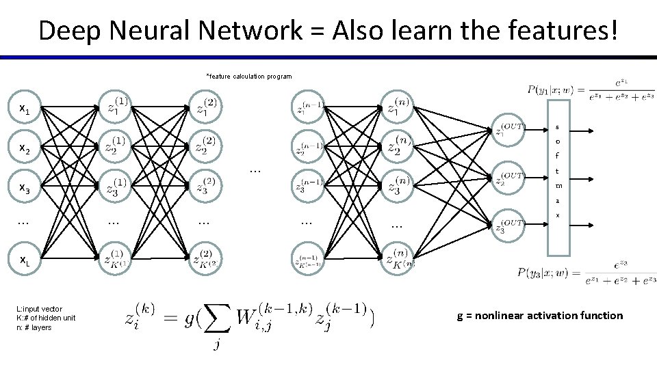
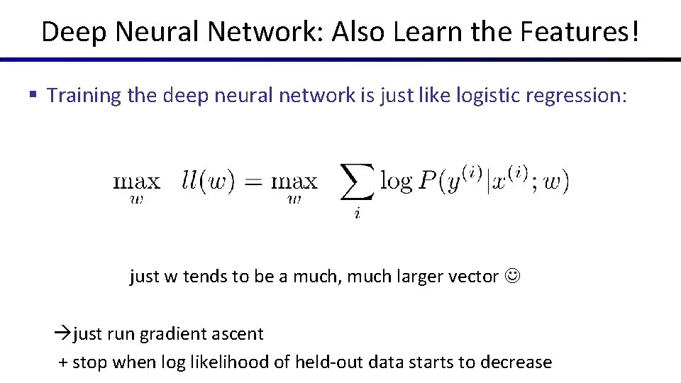
Deep Neural Network = Also learn the features! *feature calculation program x 1 x 2 … x 3 … … … s o f t m a x x. L L: input vector K: # of hidden unit n: # layers g = nonlinear activation function

Common Activation Functions [source: MIT 6. S 191 introtodeeplearning. com]

Deep Neural Network: Also Learn the Features! § Training the deep neural network is just like logistic regression: just w tends to be a much, much larger vector just run gradient ascent + stop when log likelihood of held-out data starts to decrease

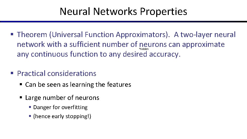
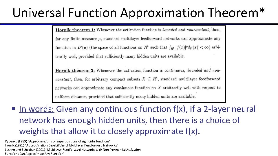
Neural Networks Properties § Theorem (Universal Function Approximators). A two-layer neural network with a sufficient number of neurons can approximate any continuous function to any desired accuracy. *hidden § Practical considerations § Can be seen as learning the features § Large number of neurons § Danger for overfitting § (hence early stopping!)

Universal Function Approximation Theorem* § In words: Given any continuous function f(x), if a 2 -layer neural network has enough hidden units, then there is a choice of weights that allow it to closely approximate f(x). Cybenko (1989) “Approximations by superpositions of sigmoidal functions” Hornik (1991) “Approximation Capabilities of Multilayer Feedforward Networks” Leshno and Schocken (1991) ”Multilayer Feedforward Networks with Non-Polynomial Activation Functions Can Approximate Any Function”

Fun Neural Net Demo Site § Demo-site: § http: //playground. tensorflow. org/

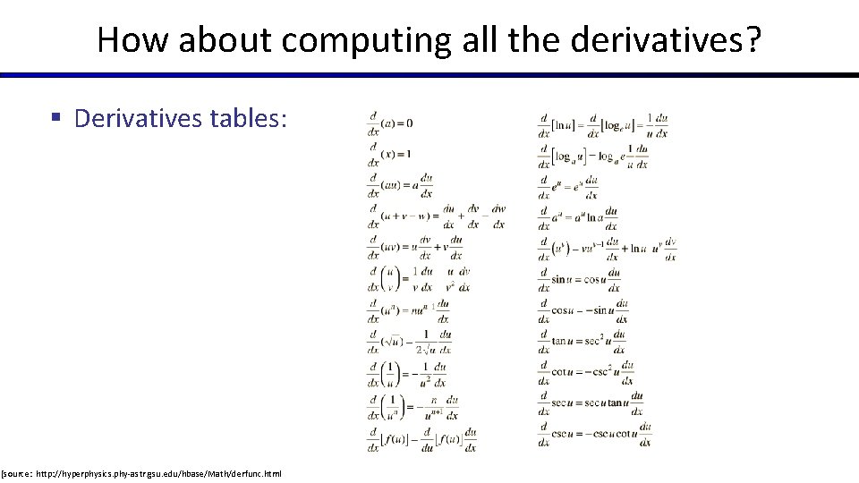
How about computing all the derivatives? § Derivatives tables: [source: http: //hyperphysics. phy-astr. gsu. edu/hbase/Math/derfunc. html

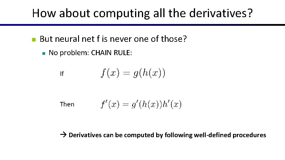
How about computing all the derivatives? n But neural net f is never one of those? n No problem: CHAIN RULE: If Then Derivatives can be computed by following well-defined procedures

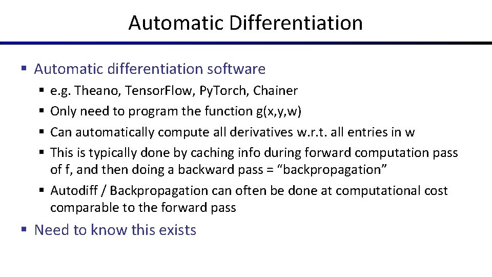
Automatic Differentiation § Automatic differentiation software e. g. Theano, Tensor. Flow, Py. Torch, Chainer Only need to program the function g(x, y, w) Can automatically compute all derivatives w. r. t. all entries in w This is typically done by caching info during forward computation pass of f, and then doing a backward pass = “backpropagation” § Autodiff / Backpropagation can often be done at computational cost comparable to the forward pass § § § Need to know this exists

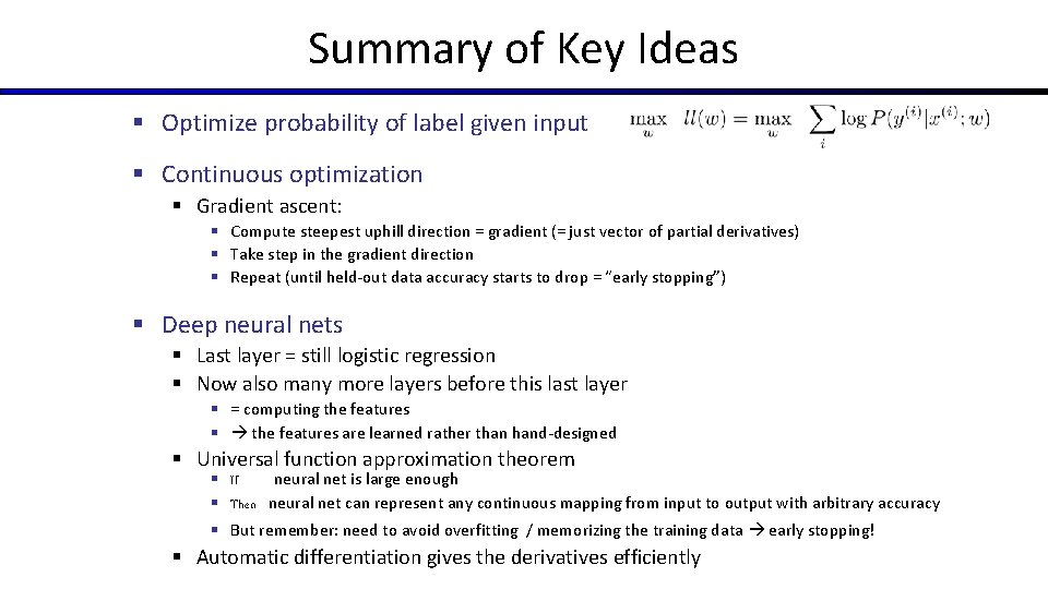
Summary of Key Ideas § Optimize probability of label given input § Continuous optimization § Gradient ascent: § Compute steepest uphill direction = gradient (= just vector of partial derivatives) § Take step in the gradient direction § Repeat (until held-out data accuracy starts to drop = “early stopping”) § Deep neural nets § Last layer = still logistic regression § Now also many more layers before this last layer § = computing the features § the features are learned rather than hand-designed § Universal function approximation theorem § If neural net is large enough § Then neural net can represent any continuous mapping from input to output with arbitrary accuracy § But remember: need to avoid overfitting / memorizing the training data early stopping! § Automatic differentiation gives the derivatives efficiently