Introduction to recognition Source Charley Harper Outline Overview

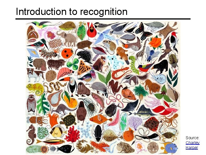
Introduction to recognition Source: Charley Harper

Outline • Overview of recognition tasks • A statistical learning approach • “Classic” or “shallow” recognition pipeline • • “Bag of features” representation Classifiers: nearest neighbor, linear, SVM • After that: neural networks, “deep” recognition pipeline

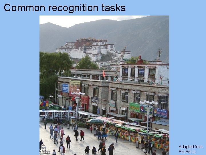
Common recognition tasks Adapted from Fei-Fei Li

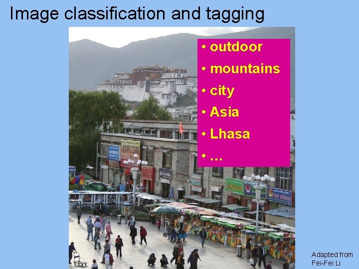
Image classification and tagging • outdoor • mountains • city • Asia • Lhasa • … Adapted from Fei-Fei Li

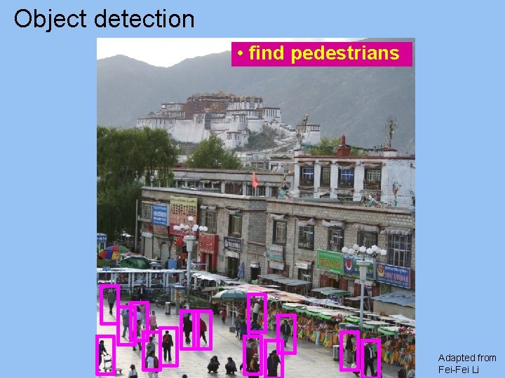
Object detection • find pedestrians Adapted from Fei-Fei Li

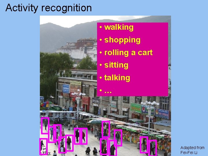
Activity recognition • walking • shopping • rolling a cart • sitting • talking • … Adapted from Fei-Fei Li

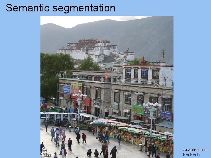
Semantic segmentation Adapted from Fei-Fei Li

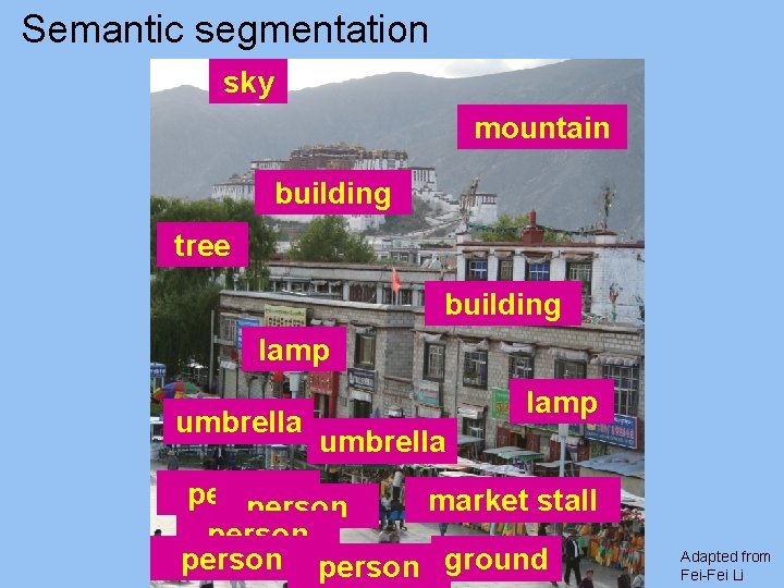
Semantic segmentation sky mountain building tree building lamp umbrella person market stall person ground Adapted from Fei-Fei Li

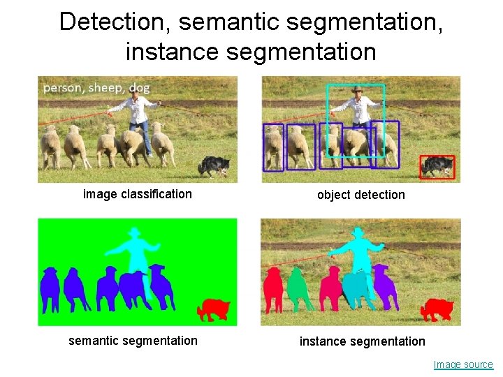
Detection, semantic segmentation, instance segmentation image classification semantic segmentation object detection instance segmentation Image source

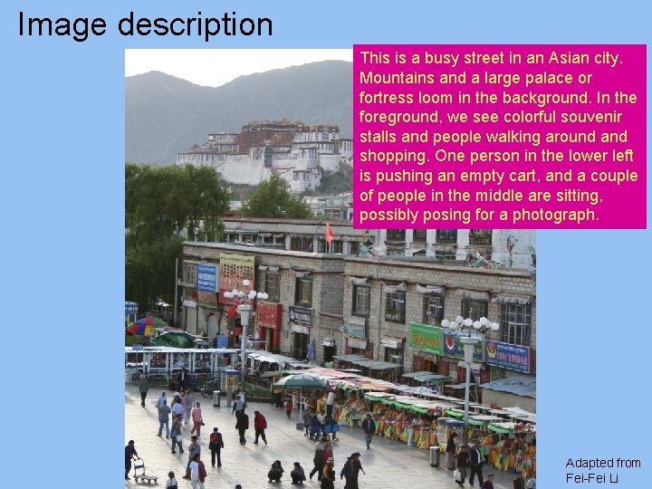
Image description This is a busy street in an Asian city. Mountains and a large palace or fortress loom in the background. In the foreground, we see colorful souvenir stalls and people walking around and shopping. One person in the lower left is pushing an empty cart, and a couple of people in the middle are sitting, possibly posing for a photograph. Adapted from Fei-Fei Li

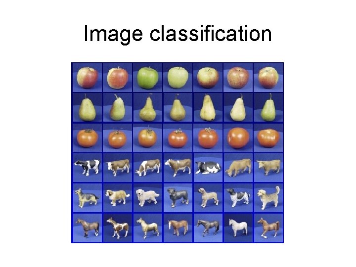
Image classification

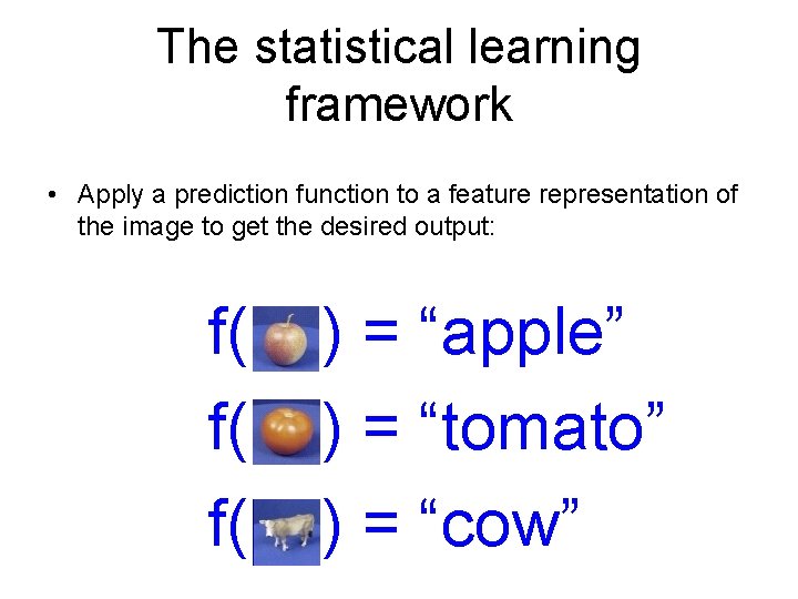
The statistical learning framework • Apply a prediction function to a feature representation of the image to get the desired output: f( f( f( ) = “apple” ) = “tomato” ) = “cow”

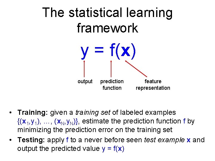
The statistical learning framework y = f(x) output prediction function feature representation • Training: given a training set of labeled examples {(x 1, y 1), …, (x. N, y. N)}, estimate the prediction function f by minimizing the prediction error on the training set • Testing: apply f to a never before seen test example x and output the predicted value y = f(x)

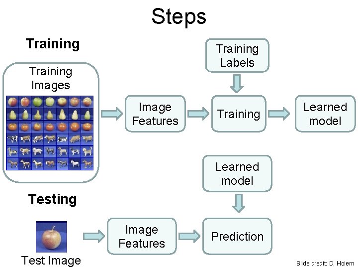
Steps Training Labels Training Images Image Features Training Learned model Testing Image Features Test Image Prediction Slide credit: D. Hoiem

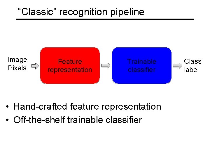
“Classic” recognition pipeline Image Pixels Feature representation Trainable classifier • Hand-crafted feature representation • Off-the-shelf trainable classifier Class label

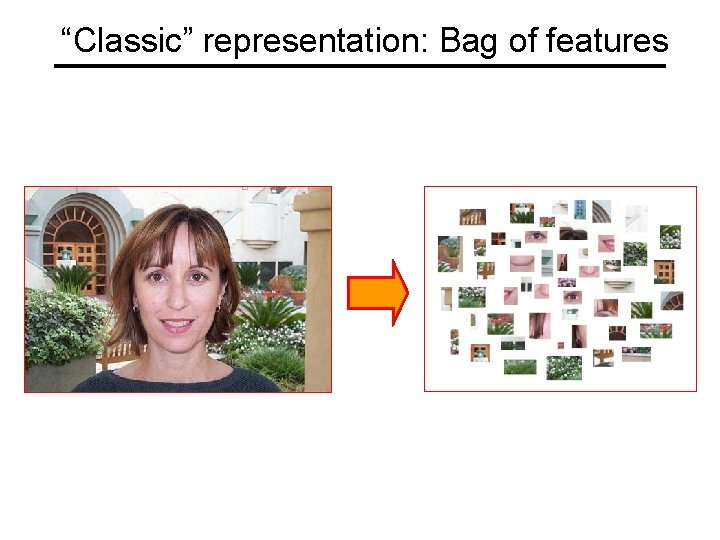
“Classic” representation: Bag of features

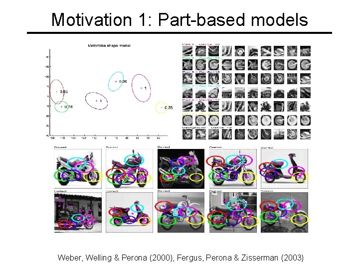
Motivation 1: Part-based models Weber, Welling & Perona (2000), Fergus, Perona & Zisserman (2003)

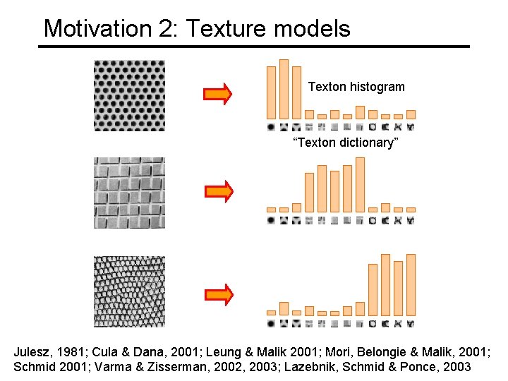
Motivation 2: Texture models Texton histogram “Texton dictionary” Julesz, 1981; Cula & Dana, 2001; Leung & Malik 2001; Mori, Belongie & Malik, 2001; Schmid 2001; Varma & Zisserman, 2002, 2003; Lazebnik, Schmid & Ponce, 2003

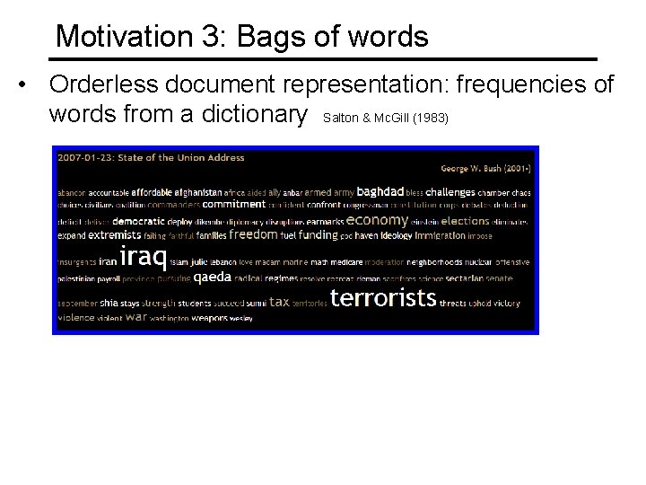
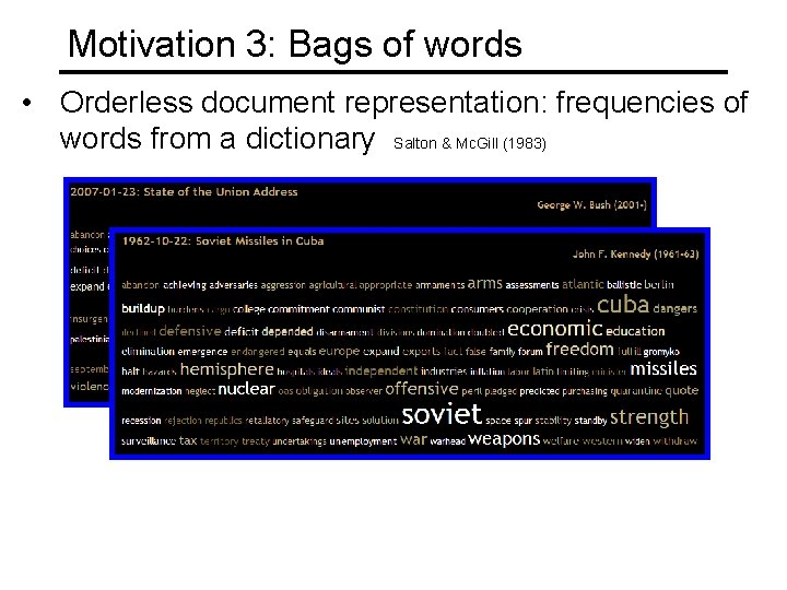
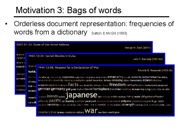
Motivation 3: Bags of words • Orderless document representation: frequencies of words from a dictionary Salton & Mc. Gill (1983)

Motivation 3: Bags of words • Orderless document representation: frequencies of words from a dictionary Salton & Mc. Gill (1983) US Presidential Speeches Tag Cloud http: //chir. ag/projects/preztags/

Motivation 3: Bags of words • Orderless document representation: frequencies of words from a dictionary Salton & Mc. Gill (1983) US Presidential Speeches Tag Cloud http: //chir. ag/projects/preztags/

Motivation 3: Bags of words • Orderless document representation: frequencies of words from a dictionary Salton & Mc. Gill (1983) US Presidential Speeches Tag Cloud http: //chir. ag/projects/preztags/

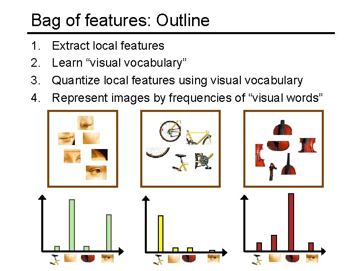
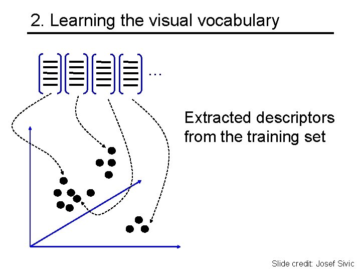
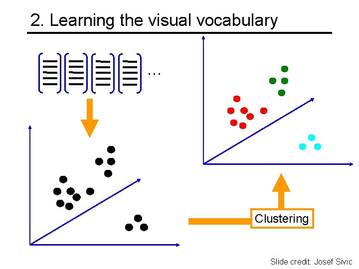
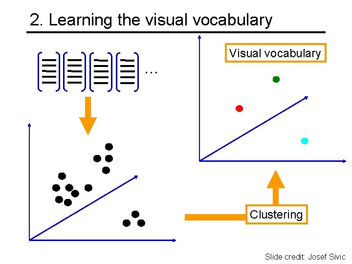
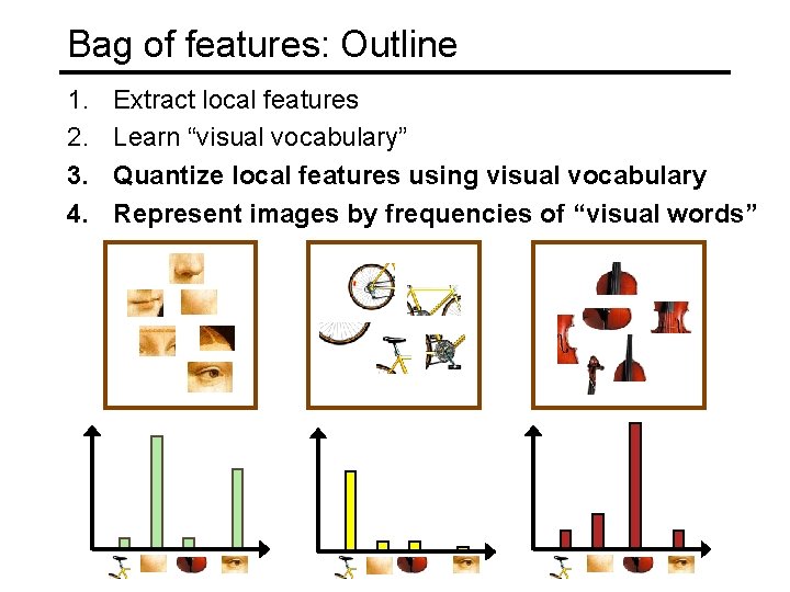
Bag of features: Outline 1. 2. 3. 4. Extract local features Learn “visual vocabulary” Quantize local features using visual vocabulary Represent images by frequencies of “visual words”

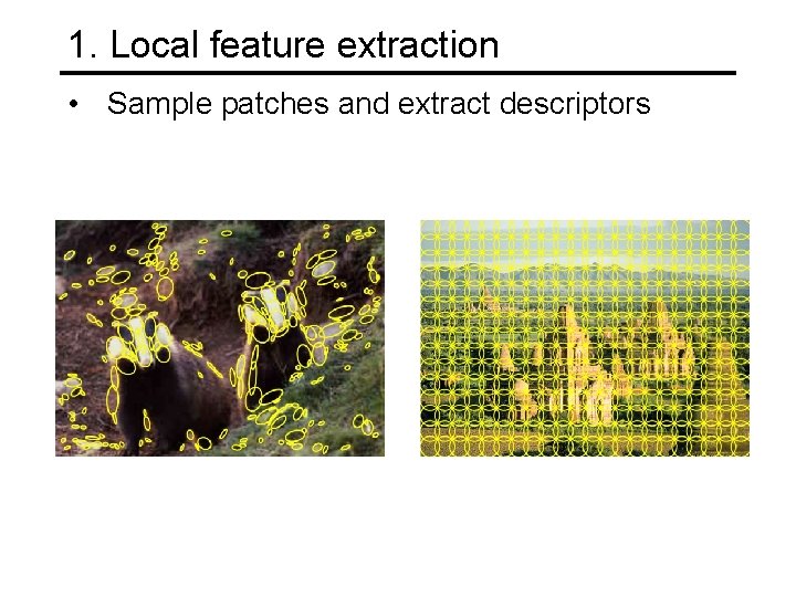
1. Local feature extraction • Sample patches and extract descriptors

2. Learning the visual vocabulary … Extracted descriptors from the training set Slide credit: Josef Sivic

2. Learning the visual vocabulary … Clustering Slide credit: Josef Sivic

2. Learning the visual vocabulary … Visual vocabulary Clustering Slide credit: Josef Sivic

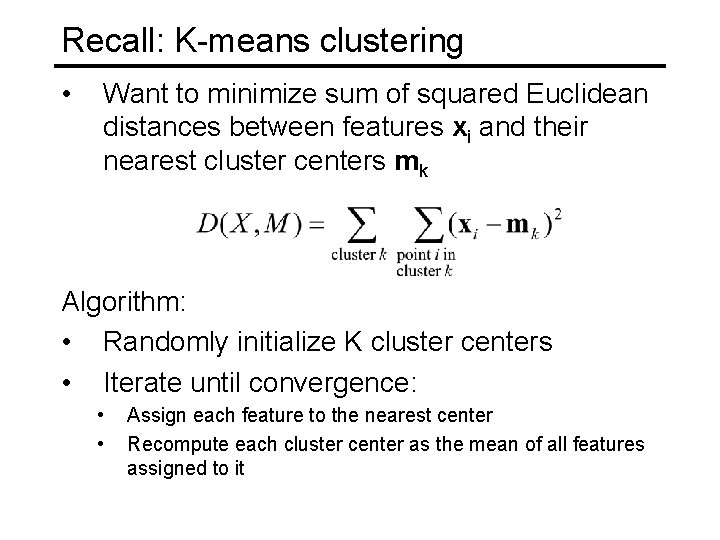
Recall: K-means clustering • Want to minimize sum of squared Euclidean distances between features xi and their nearest cluster centers mk Algorithm: • Randomly initialize K cluster centers • Iterate until convergence: • • Assign each feature to the nearest center Recompute each cluster center as the mean of all features assigned to it

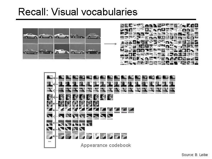
Recall: Visual vocabularies … Appearance codebook Source: B. Leibe

Bag of features: Outline 1. 2. 3. 4. Extract local features Learn “visual vocabulary” Quantize local features using visual vocabulary Represent images by frequencies of “visual words”

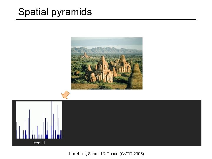
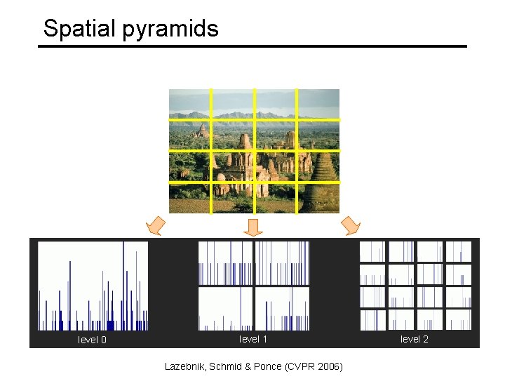
Spatial pyramids level 0 Lazebnik, Schmid & Ponce (CVPR 2006)

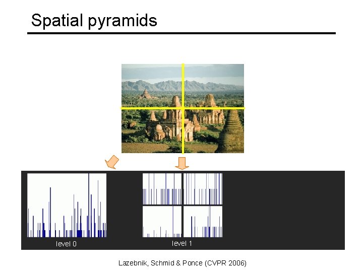
Spatial pyramids level 0 level 1 Lazebnik, Schmid & Ponce (CVPR 2006)

Spatial pyramids level 0 level 1 Lazebnik, Schmid & Ponce (CVPR 2006) level 2

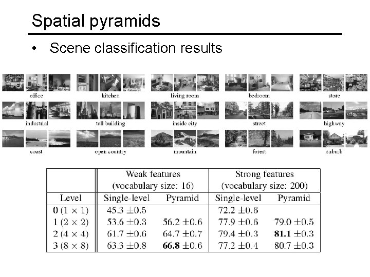
Spatial pyramids • Scene classification results

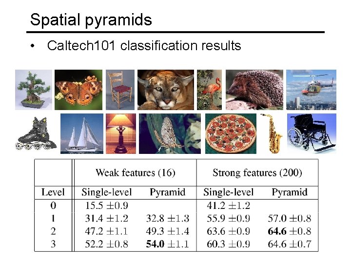
Spatial pyramids • Caltech 101 classification results

“Classic” recognition pipeline Image Pixels Feature representation Trainable classifier • Hand-crafted feature representation • Off-the-shelf trainable classifier Class label

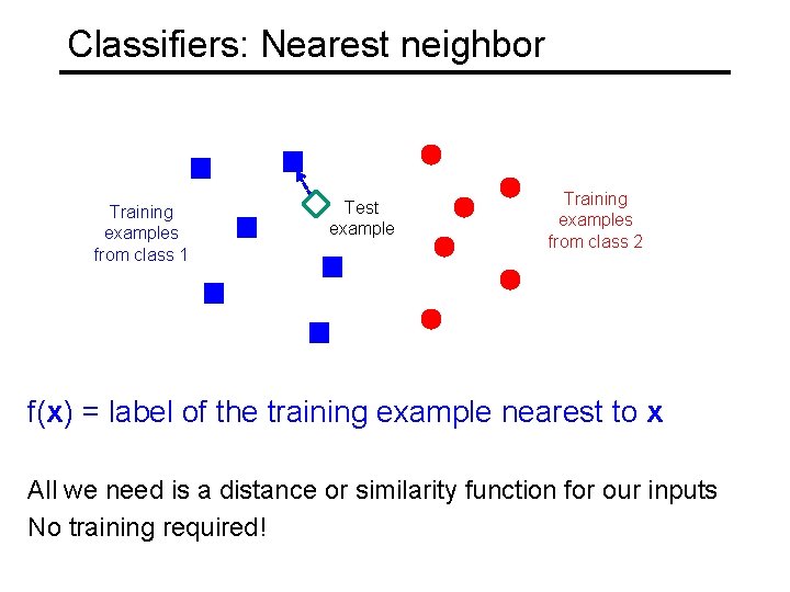
Classifiers: Nearest neighbor Training examples from class 1 Test example Training examples from class 2 f(x) = label of the training example nearest to x All we need is a distance or similarity function for our inputs No training required!

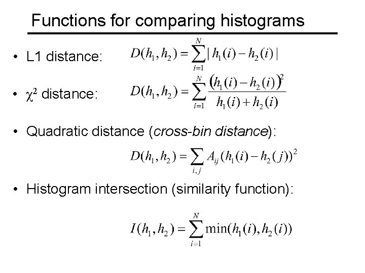
Functions for comparing histograms • L 1 distance: • χ2 distance: • Quadratic distance (cross-bin distance): • Histogram intersection (similarity function):

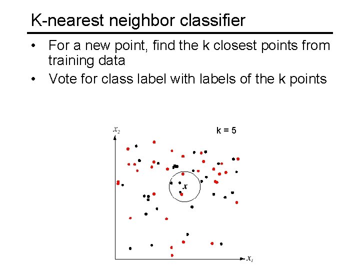
K-nearest neighbor classifier • For a new point, find the k closest points from training data • Vote for class label with labels of the k points k=5

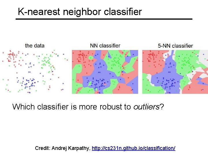
K-nearest neighbor classifier Which classifier is more robust to outliers? Credit: Andrej Karpathy, http: //cs 231 n. github. io/classification/

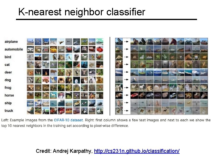
K-nearest neighbor classifier Credit: Andrej Karpathy, http: //cs 231 n. github. io/classification/

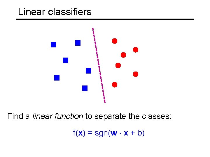
Linear classifiers Find a linear function to separate the classes: f(x) = sgn(w x + b)

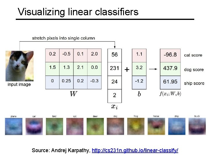
Visualizing linear classifiers Source: Andrej Karpathy, http: //cs 231 n. github. io/linear-classify/

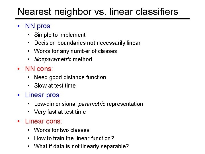
Nearest neighbor vs. linear classifiers • NN pros: • • Simple to implement Decision boundaries not necessarily linear Works for any number of classes Nonparametric method • NN cons: • Need good distance function • Slow at test time • Linear pros: • Low-dimensional parametric representation • Very fast at test time • Linear cons: • Works for two classes • How to train the linear function? • What if data is not linearly separable?

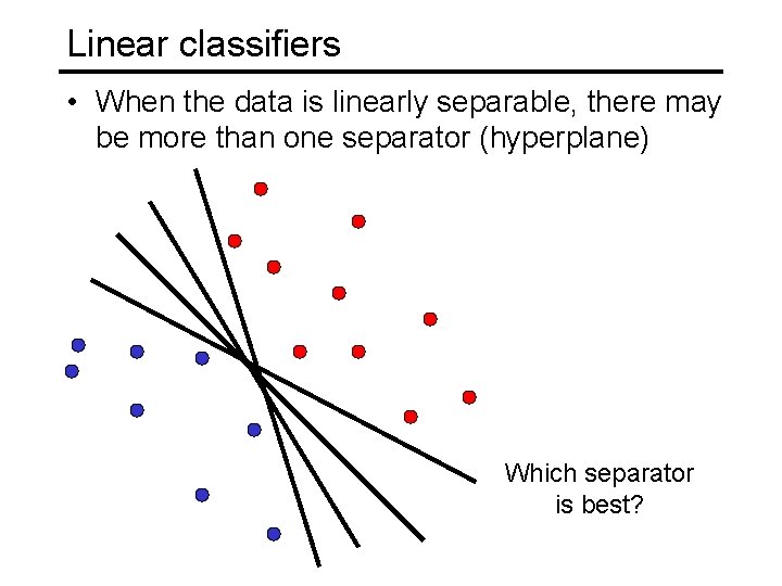
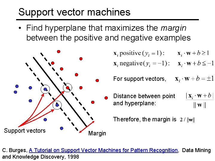
Linear classifiers • When the data is linearly separable, there may be more than one separator (hyperplane) Which separator is best?

Support vector machines • Find hyperplane that maximizes the margin between the positive and negative examples For support vectors, Distance between point and hyperplane: Therefore, the margin is 2 / ||w|| Support vectors Margin C. Burges, A Tutorial on Support Vector Machines for Pattern Recognition, Data Mining and Knowledge Discovery, 1998

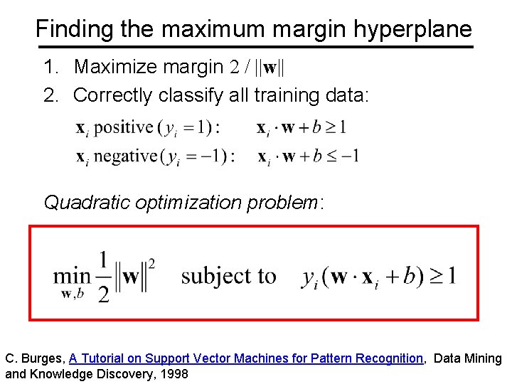
Finding the maximum margin hyperplane 1. Maximize margin 2 / ||w|| 2. Correctly classify all training data: Quadratic optimization problem: C. Burges, A Tutorial on Support Vector Machines for Pattern Recognition, Data Mining and Knowledge Discovery, 1998

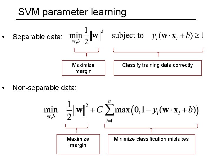
SVM parameter learning • Separable data: Maximize margin • Classify training data correctly Non-separable data: Maximize margin Minimize classification mistakes

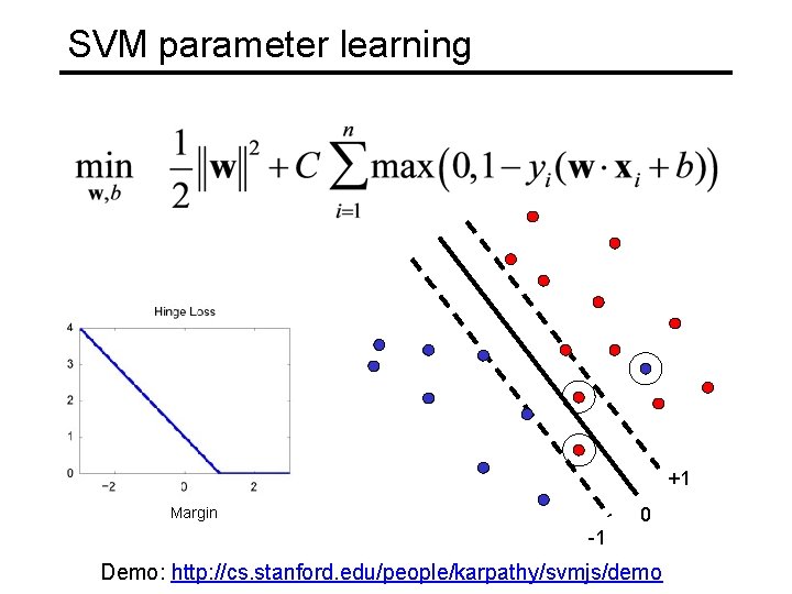
SVM parameter learning +1 0 Margin -1 Demo: http: //cs. stanford. edu/people/karpathy/svmjs/demo

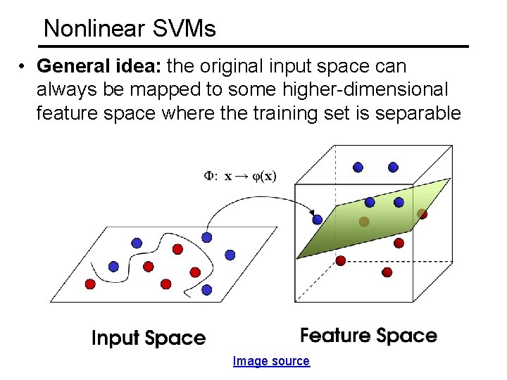
Nonlinear SVMs • General idea: the original input space can always be mapped to some higher-dimensional feature space where the training set is separable Φ: x → φ(x) Image source

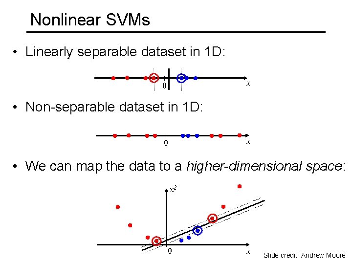
Nonlinear SVMs • Linearly separable dataset in 1 D: x 0 • Non-separable dataset in 1 D: x 0 • We can map the data to a higher-dimensional space: x 2 0 x Slide credit: Andrew Moore

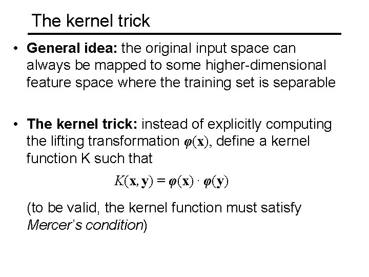
The kernel trick • General idea: the original input space can always be mapped to some higher-dimensional feature space where the training set is separable • The kernel trick: instead of explicitly computing the lifting transformation φ(x), define a kernel function K such that K(x , y) = φ(x) · φ(y) (to be valid, the kernel function must satisfy Mercer’s condition)

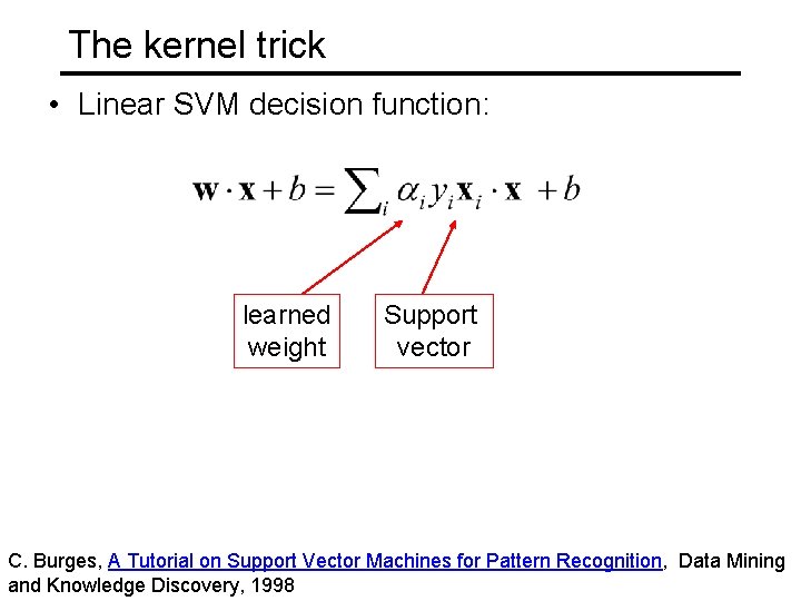
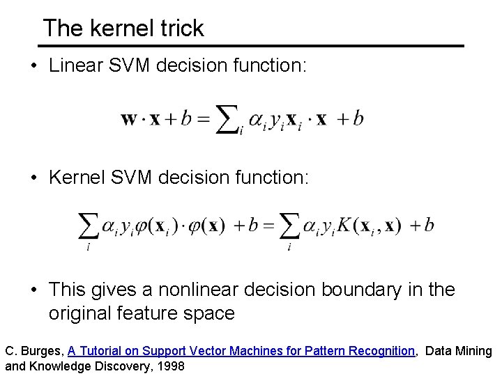
The kernel trick • Linear SVM decision function: learned weight Support vector C. Burges, A Tutorial on Support Vector Machines for Pattern Recognition, Data Mining and Knowledge Discovery, 1998

The kernel trick • Linear SVM decision function: • Kernel SVM decision function: • This gives a nonlinear decision boundary in the original feature space C. Burges, A Tutorial on Support Vector Machines for Pattern Recognition, Data Mining and Knowledge Discovery, 1998

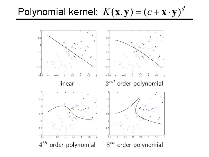
Polynomial kernel:

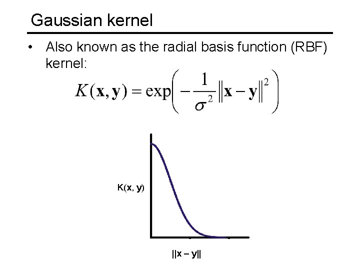
Gaussian kernel • Also known as the radial basis function (RBF) kernel: K(x, y) ||x – y||

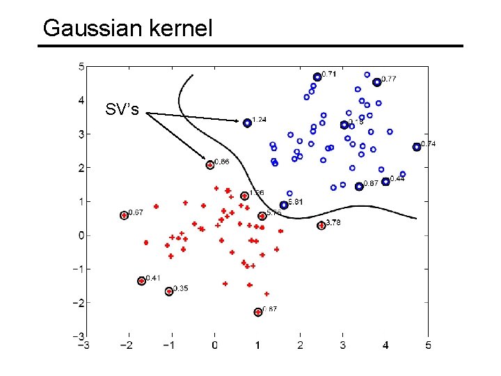
Gaussian kernel SV’s

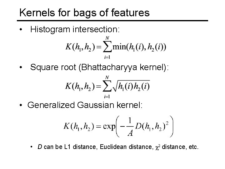
Kernels for bags of features • Histogram intersection: • Square root (Bhattacharyya kernel): • Generalized Gaussian kernel: • D can be L 1 distance, Euclidean distance, χ2 distance, etc.

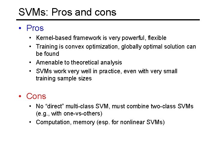
SVMs: Pros and cons • Pros • Kernel-based framework is very powerful, flexible • Training is convex optimization, globally optimal solution can be found • Amenable to theoretical analysis • SVMs work very well in practice, even with very small training sample sizes • Cons • No “direct” multi-class SVM, must combine two-class SVMs (e. g. , with one-vs-others) • Computation, memory (esp. for nonlinear SVMs)