Introduction to Logistic Regression EPI 204 Quantitative Epidemiology

Introduction to Logistic Regression EPI 204 Quantitative Epidemiology III Statistical Models April 2, 2019 EPI 204 Quantitative Epidemiology III 1

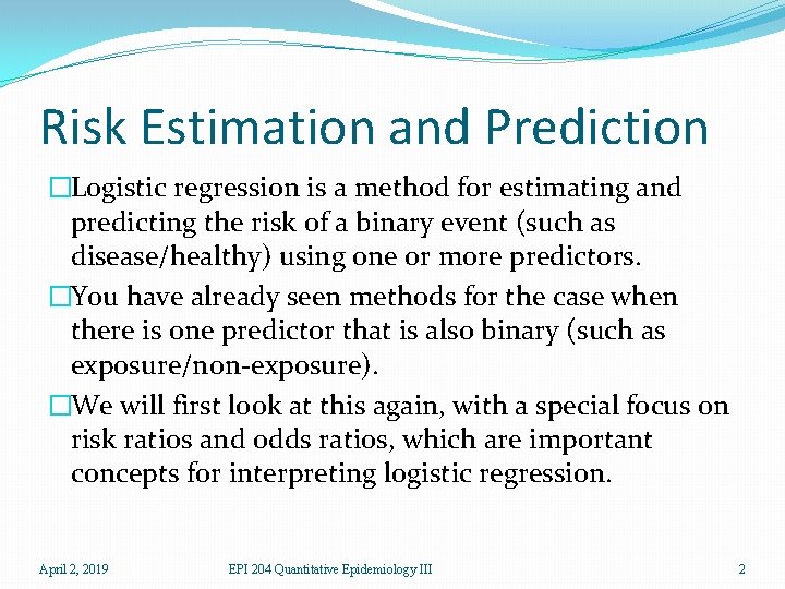
Risk Estimation and Prediction �Logistic regression is a method for estimating and predicting the risk of a binary event (such as disease/healthy) using one or more predictors. �You have already seen methods for the case when there is one predictor that is also binary (such as exposure/non-exposure). �We will first look at this again, with a special focus on risk ratios and odds ratios, which are important concepts for interpreting logistic regression. April 2, 2019 EPI 204 Quantitative Epidemiology III 2

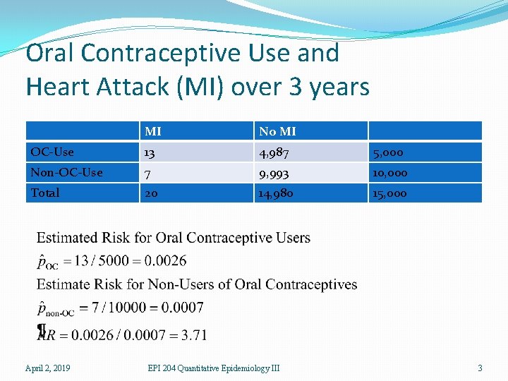
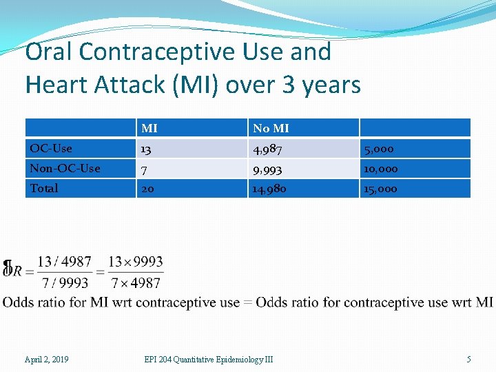
Oral Contraceptive Use and Heart Attack (MI) over 3 years MI No MI OC-Use 13 4, 987 5, 000 Non-OC-Use 7 9, 993 10, 000 Total 20 14, 980 15, 000 April 2, 2019 EPI 204 Quantitative Epidemiology III 3

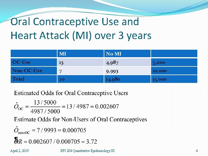
Oral Contraceptive Use and Heart Attack (MI) over 3 years MI No MI OC-Use 13 4, 987 5, 000 Non-OC-Use 7 9, 993 10, 000 Total 20 14, 980 15, 000 April 2, 2019 EPI 204 Quantitative Epidemiology III 4

Oral Contraceptive Use and Heart Attack (MI) over 3 years MI No MI OC-Use 13 4, 987 5, 000 Non-OC-Use 7 9, 993 10, 000 Total 20 14, 980 15, 000 April 2, 2019 EPI 204 Quantitative Epidemiology III 5

Effect of Study Design �The table is from a follow-up study in which two populations were followed and the number of MI’s was observed. �The risk is P(MI|OC) and P(MI|non-OC) and this is valid for this design. �But suppose we had a case-control study in which we had 100 women with MI and selected a comparison group of 100 women without MI (matched on age, etc. ). �Then MI is not random, and we cannot compute P(MI|OC) and we cannot compute the risk ratio. April 2, 2019 EPI 204 Quantitative Epidemiology III 6

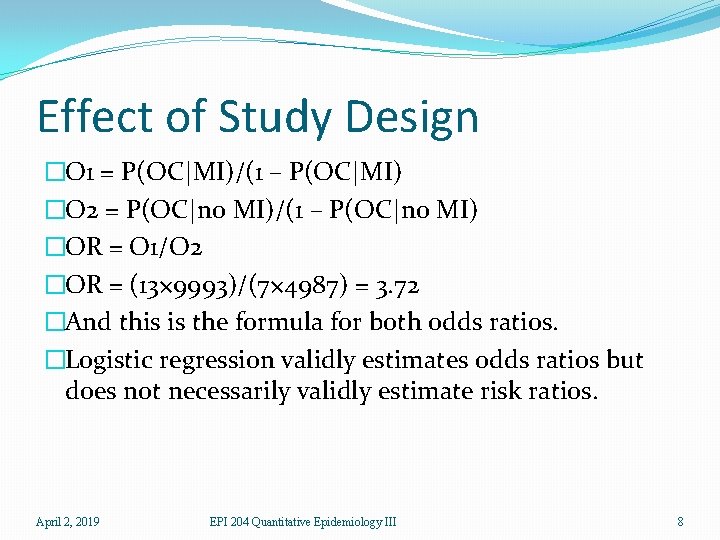
Effect of Study Design �The odds ratio however can be computed. �The disease odds ratio is the odds for the disease in the exposed group divided by the odds for the disease in the unexposed group, and we cannot validly compute and use these separate parts. �But we can validly compute and use the exposure odds ratio, which is the odds for exposure in the disease group divided by the odds for exposure in the non-diseased group (because exposure can be treated as random). �And these are numerically the same. April 2, 2019 EPI 204 Quantitative Epidemiology III 7

Effect of Study Design �O 1 = P(OC|MI)/(1 – P(OC|MI) �O 2 = P(OC|no MI)/(1 – P(OC|no MI) �OR = O 1/O 2 �OR = (13× 9993)/(7× 4987) = 3. 72 �And this is the formula for both odds ratios. �Logistic regression validly estimates odds ratios but does not necessarily validly estimate risk ratios. April 2, 2019 EPI 204 Quantitative Epidemiology III 8

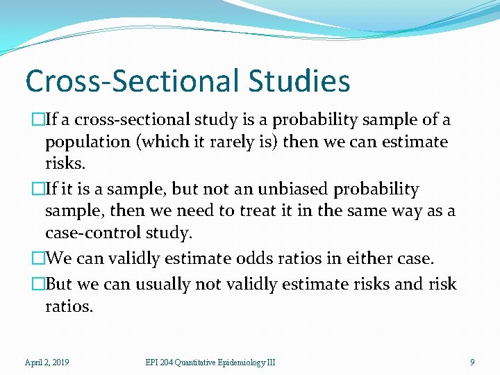
Cross-Sectional Studies �If a cross-sectional study is a probability sample of a population (which it rarely is) then we can estimate risks. �If it is a sample, but not an unbiased probability sample, then we need to treat it in the same way as a case-control study. �We can validly estimate odds ratios in either case. �But we can usually not validly estimate risks and risk ratios. April 2, 2019 EPI 204 Quantitative Epidemiology III 9

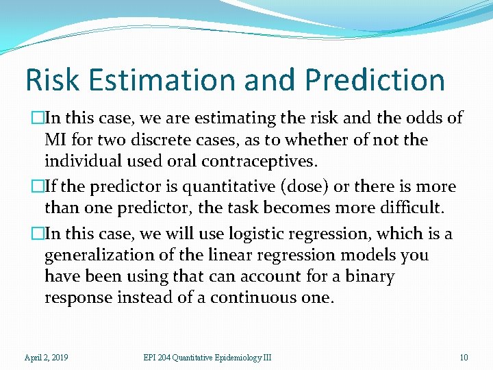
Risk Estimation and Prediction �In this case, we are estimating the risk and the odds of MI for two discrete cases, as to whether of not the individual used oral contraceptives. �If the predictor is quantitative (dose) or there is more than one predictor, the task becomes more difficult. �In this case, we will use logistic regression, which is a generalization of the linear regression models you have been using that can account for a binary response instead of a continuous one. April 2, 2019 EPI 204 Quantitative Epidemiology III 10

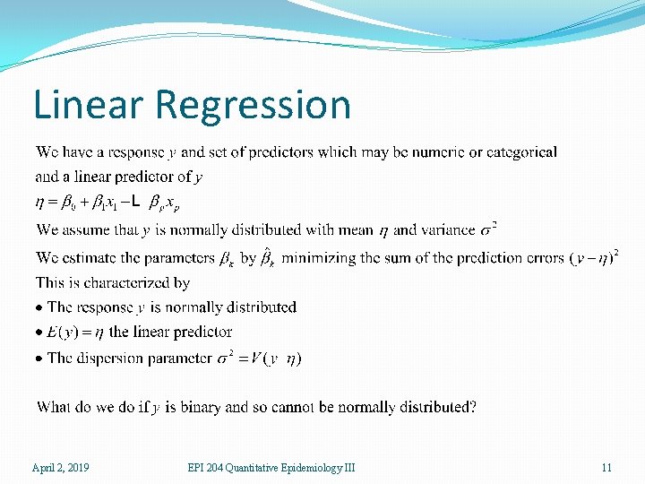
Linear Regression April 2, 2019 EPI 204 Quantitative Epidemiology III 11

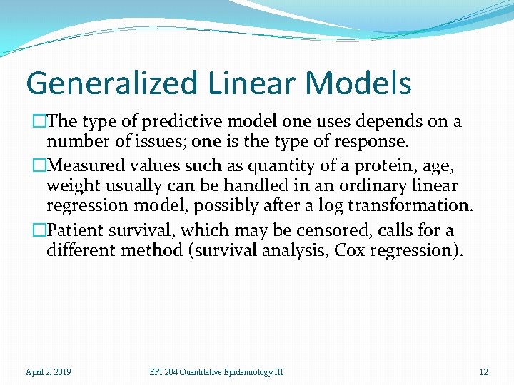
Generalized Linear Models �The type of predictive model one uses depends on a number of issues; one is the type of response. �Measured values such as quantity of a protein, age, weight usually can be handled in an ordinary linear regression model, possibly after a log transformation. �Patient survival, which may be censored, calls for a different method (survival analysis, Cox regression). April 2, 2019 EPI 204 Quantitative Epidemiology III 12

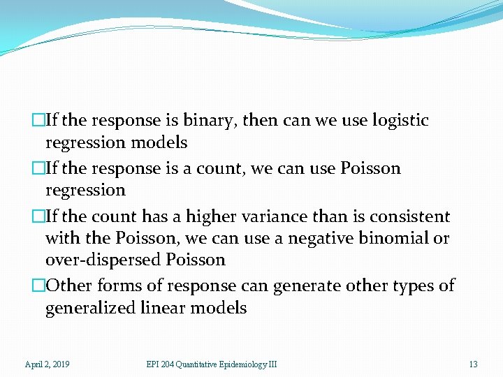
�If the response is binary, then can we use logistic regression models �If the response is a count, we can use Poisson regression �If the count has a higher variance than is consistent with the Poisson, we can use a negative binomial or over-dispersed Poisson �Other forms of response can generate other types of generalized linear models April 2, 2019 EPI 204 Quantitative Epidemiology III 13

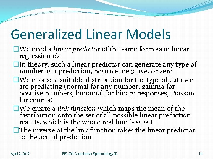
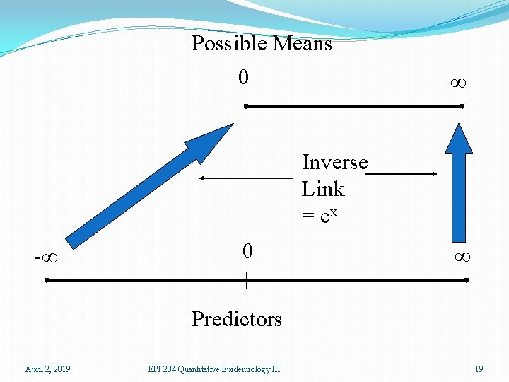
Generalized Linear Models �We need a linear predictor of the same form as in linear regression βx �In theory, such a linear predictor can generate any type of number as a prediction, positive, negative, or zero �We choose a suitable distribution for the type of data we are predicting (normal for any number, gamma for positive numbers, binomial for binary responses, Poisson for counts) �We create a link function which maps the mean of the distribution onto the set of all possible linear prediction results, which is the whole real line (-∞, ∞). �The inverse of the link function takes the linear predictor to the actual prediction April 2, 2019 EPI 204 Quantitative Epidemiology III 14

�Ordinary linear regression has identity link (no transformation by the link function) and uses the normal distribution �If one is predicting an inherently positive quantity, one may want to use the log link since ex is always positive. �An alternative to using a generalized linear model with an log link, is to transform the data using the log. This is a device that works well with measurement data and may be usable in other cases, but it cannot be used for 0/1 data or count data that may be 0. April 2, 2019 EPI 204 Quantitative Epidemiology III 15

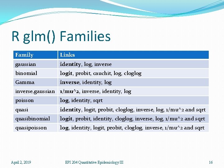
R glm() Families Family Links gaussian identity, log, inverse binomial logit, probit, cauchit, log, cloglog Gamma inverse, identity, log inverse. gaussian 1/mu^2, inverse, identity, log poisson log, identity, sqrt quasi identity, logit, probit, cloglog, inverse, log, 1/mu^2 and sqrt quasibinomial logit, probit, identity, cloglog, inverse, log, 1/mu^2 and sqrt quasipoisson log, identity, logit, probit, cloglog, inverse, 1/mu^2 and sqrt April 2, 2019 EPI 204 Quantitative Epidemiology III 16

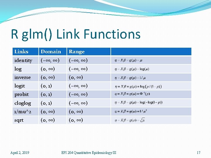
R glm() Link Functions Links Domain Range identity (−∞, ∞) log (0, ∞) (−∞, ∞) inverse (0, ∞) logit (0, 1) (−∞, ∞) probit (0, 1) (−∞, ∞) cloglog (0, 1) (−∞, ∞) 1/mu^2 (0, ∞) sqrt (0, ∞) April 2, 2019 EPI 204 Quantitative Epidemiology III 17

Possible Means 0 ∞ Link = Log -∞ 0 ∞ Predictors April 2, 2019 EPI 204 Quantitative Epidemiology III 18

Possible Means 0 ∞ Inverse Link = ex -∞ 0 ∞ Predictors April 2, 2019 EPI 204 Quantitative Epidemiology III 19

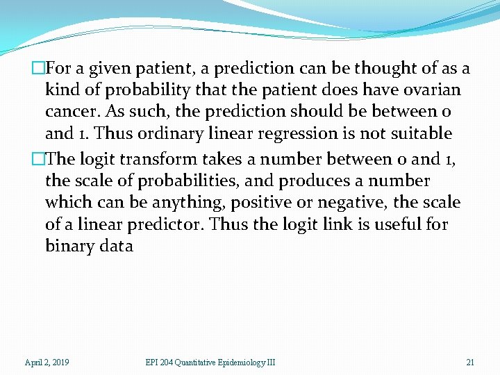
Logistic Regression �Suppose we are trying to predict a binary variable (patient has ovarian cancer or not, patient is responding to therapy or not) �We can describe this by a 0/1 variable in which the value 1 is used for one response (patient has ovarian cancer) and 0 for the other (patient does not have ovarian cancer �We can then try to predict this response April 2, 2019 EPI 204 Quantitative Epidemiology III 20

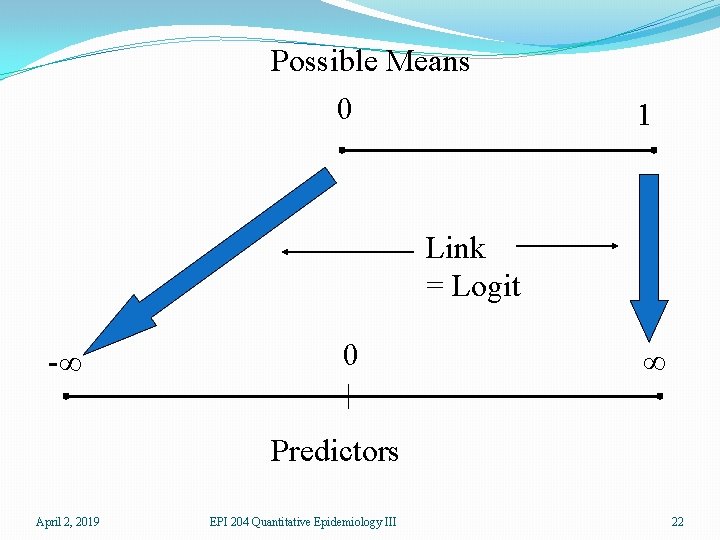
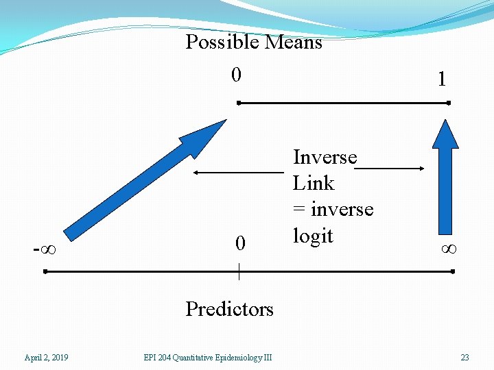
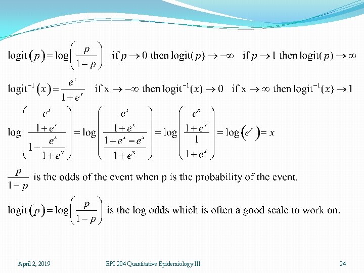
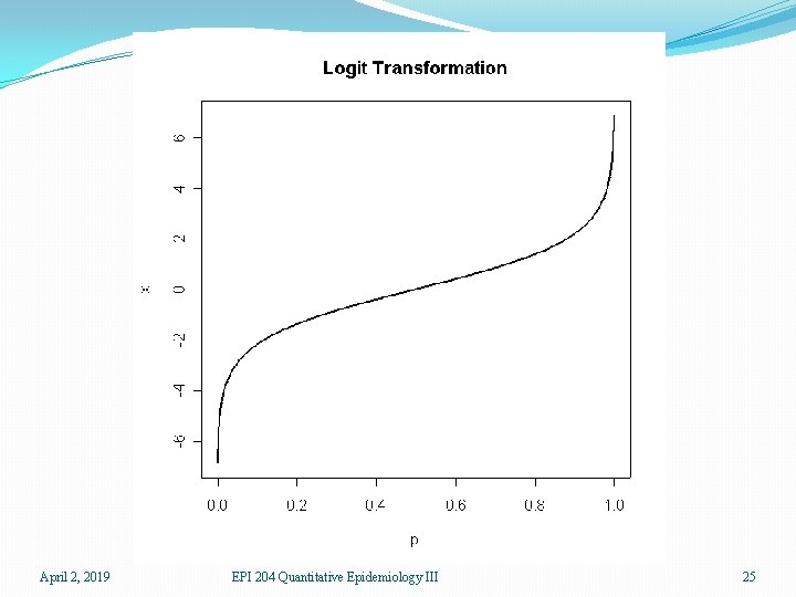
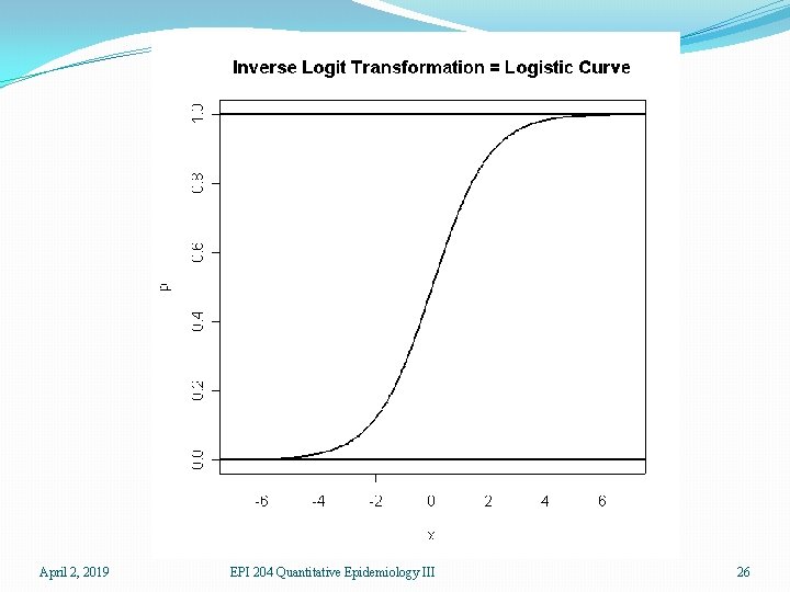
�For a given patient, a prediction can be thought of as a kind of probability that the patient does have ovarian cancer. As such, the prediction should be between 0 and 1. Thus ordinary linear regression is not suitable �The logit transform takes a number between 0 and 1, the scale of probabilities, and produces a number which can be anything, positive or negative, the scale of a linear predictor. Thus the logit link is useful for binary data April 2, 2019 EPI 204 Quantitative Epidemiology III 21

Possible Means 0 1 Link = Logit -∞ 0 ∞ Predictors April 2, 2019 EPI 204 Quantitative Epidemiology III 22

Possible Means 0 -∞ 0 Inverse Link = inverse logit 1 ∞ Predictors April 2, 2019 EPI 204 Quantitative Epidemiology III 23

April 2, 2019 EPI 204 Quantitative Epidemiology III 24

April 2, 2019 EPI 204 Quantitative Epidemiology III 25

April 2, 2019 EPI 204 Quantitative Epidemiology III 26

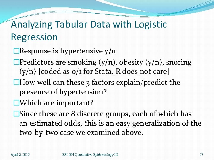
Analyzing Tabular Data with Logistic Regression �Response is hypertensive y/n �Predictors are smoking (y/n), obesity (y/n), snoring (y/n) [coded as 0/1 for Stata, R does not care] �How well can these 3 factors explain/predict the presence of hypertension? �Which are important? �Since these are 8 discrete groups, each of which has an estimated odds, this is an easy generalization of the two-by-two case we examined above. April 2, 2019 EPI 204 Quantitative Epidemiology III 27

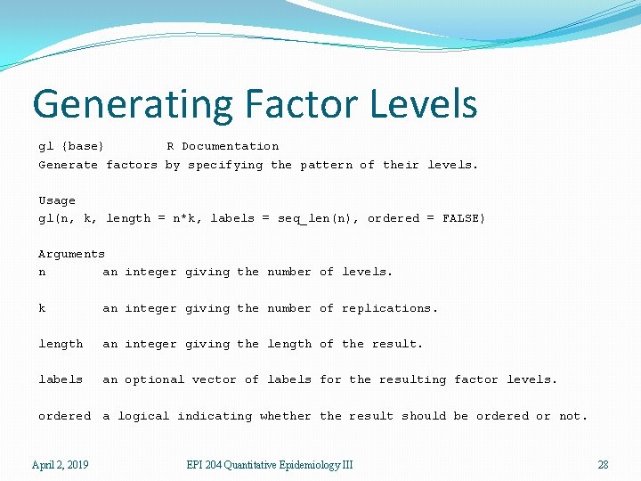
Generating Factor Levels gl {base} R Documentation Generate factors by specifying the pattern of their levels. Usage gl(n, k, length = n*k, labels = seq_len(n), ordered = FALSE) Arguments n an integer giving the number of levels. k an integer giving the number of replications. length an integer giving the length of the result. labels an optional vector of labels for the resulting factor levels. ordered a logical indicating whether the result should be ordered or not. April 2, 2019 EPI 204 Quantitative Epidemiology III 28

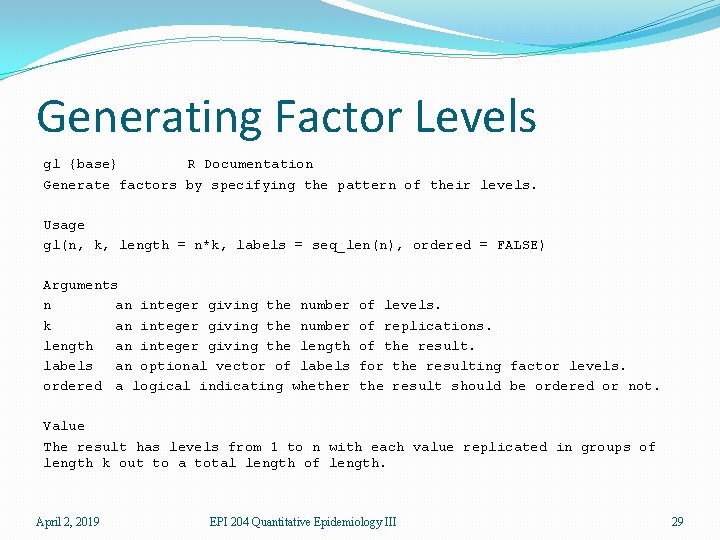
Generating Factor Levels gl {base} R Documentation Generate factors by specifying the pattern of their levels. Usage gl(n, k, length = n*k, labels = seq_len(n), ordered = FALSE) Arguments n an integer giving the number k an integer giving the number length an integer giving the length labels an optional vector of labels ordered a logical indicating whether of levels. of replications. of the result. for the resulting factor levels. the result should be ordered or not. Value The result has levels from 1 to n with each value replicated in groups of length k out to a total length of length. April 2, 2019 EPI 204 Quantitative Epidemiology III 29

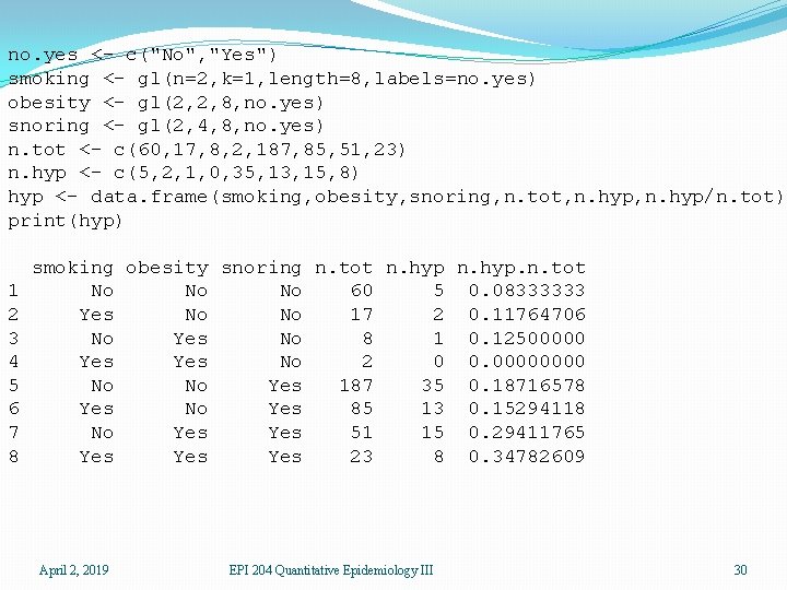
no. yes <- c("No", "Yes") smoking <- gl(n=2, k=1, length=8, labels=no. yes) obesity <- gl(2, 2, 8, no. yes) snoring <- gl(2, 4, 8, no. yes) n. tot <- c(60, 17, 8, 2, 187, 85, 51, 23) n. hyp <- c(5, 2, 1, 0, 35, 13, 15, 8) hyp <- data. frame(smoking, obesity, snoring, n. tot, n. hyp/n. tot) print(hyp) 1 2 3 4 5 6 7 8 smoking obesity snoring n. tot n. hyp. n. tot No No No 60 5 0. 08333333 Yes No No 17 2 0. 11764706 No Yes No 8 1 0. 12500000 Yes No 2 0 0. 0000 No No Yes 187 35 0. 18716578 Yes No Yes 85 13 0. 15294118 No Yes 51 15 0. 29411765 Yes Yes 23 8 0. 34782609 April 2, 2019 EPI 204 Quantitative Epidemiology III 30

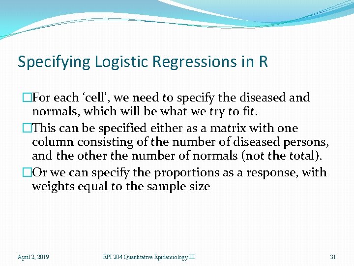
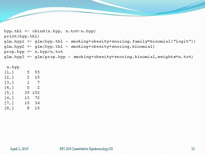
Specifying Logistic Regressions in R �For each ‘cell’, we need to specify the diseased and normals, which will be what we try to fit. �This can be specified either as a matrix with one column consisting of the number of diseased persons, and the other the number of normals (not the total). �Or we can specify the proportions as a response, with weights equal to the sample size April 2, 2019 EPI 204 Quantitative Epidemiology III 31

hyp. tbl <- cbind(n. hyp, n. tot-n. hyp) print(hyp. tbl) glm. hyp 1 <- glm(hyp. tbl ~ smoking+obesity+snoring, family=binomial("logit")) glm. hyp 2 <- glm(hyp. tbl ~ smoking+obesity+snoring, binomial) prop. hyp <- n. hyp/n. tot glm. hyp 3 <- glm(prop. hyp ~ smoking+obesity+snoring, binomial, weights=n. tot) n. hyp [1, ] [2, ] [3, ] [4, ] [5, ] [6, ] [7, ] [8, ] 5 55 2 15 1 7 0 2 35 152 13 72 15 36 8 15 April 2, 2019 EPI 204 Quantitative Epidemiology III 32

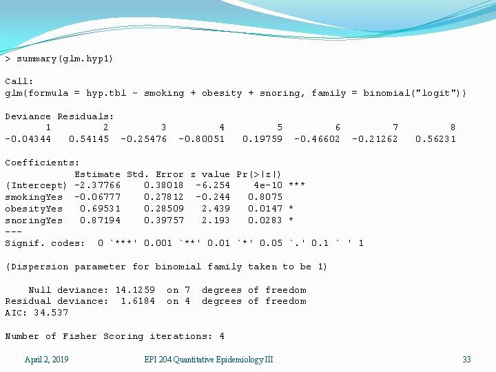
> summary(glm. hyp 1) Call: glm(formula = hyp. tbl ~ smoking + obesity + snoring, family = binomial("logit")) Deviance Residuals: 1 2 3 -0. 04344 0. 54145 -0. 25476 4 -0. 80051 5 0. 19759 6 -0. 46602 7 -0. 21262 8 0. 56231 Coefficients: Estimate Std. Error z value Pr(>|z|) (Intercept) -2. 37766 0. 38018 -6. 254 4 e-10 *** smoking. Yes -0. 06777 0. 27812 -0. 244 0. 8075 obesity. Yes 0. 69531 0. 28509 2. 439 0. 0147 * snoring. Yes 0. 87194 0. 39757 2. 193 0. 0283 * --Signif. codes: 0 `***' 0. 001 `**' 0. 01 `*' 0. 05 `. ' 0. 1 ` ' 1 (Dispersion parameter for binomial family taken to be 1) Null deviance: 14. 1259 Residual deviance: 1. 6184 AIC: 34. 537 on 4 degrees of freedom Number of Fisher Scoring iterations: 4 April 2, 2019 EPI 204 Quantitative Epidemiology III 33

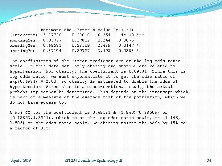
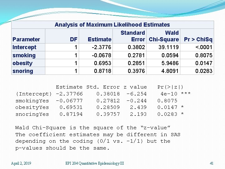
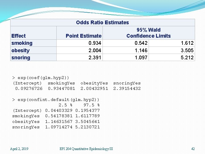
Estimate Std. Error z value Pr(>|z|) (Intercept) -2. 37766 0. 38018 -6. 254 4 e-10 *** smoking. Yes -0. 06777 0. 27812 -0. 244 0. 8075 obesity. Yes 0. 69531 0. 28509 2. 439 0. 0147 * snoring. Yes 0. 87194 0. 39757 2. 193 0. 0283 * The coefficients of the linear predictor are on the log odds ratio scale. In this data set, only obesity and snoring are related to hypertension. For obesity, the coefficient is 0. 69531. Since this is log odds ratio, we must exponentiate it to get the odds ratio of exp(0. 6931) = 2. 00, so obesity is estimated to double the odds of hypertension. Since this is a cross-sectional study, the actual probability cannot be determined. This depends on the intercept which is part of a measure of the average risk of the population, which we do not have access to. A 95% CI for the coefficient is 0. 69531 ± (1. 960)(0. 28509) or (0. 13653, 1. 2541), which is on the log odds ratio scale, or (1. 146, 3. 505) on the odds ratio scale. So obesity raises the odds by 15% to a factor of 3. 5. April 2, 2019 EPI 204 Quantitative Epidemiology III 34

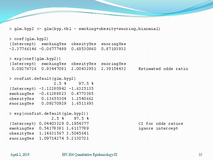
> glm. hyp 2 <- glm(hyp. tbl ~ smoking+obesity+snoring, binomial) > coef(glm. hyp 2) (Intercept) smoking. Yes -2. 37766146 -0. 06777489 obesity. Yes 0. 69530960 snoring. Yes 0. 87193932 > exp(coef(glm. hyp 2)) (Intercept) smoking. Yes 0. 09276726 0. 93447081 obesity. Yes 2. 00432951 snoring. Yes 2. 39154432 Estimated odds ratio > confint. default(glm. hyp 2) 2. 5 % 97. 5 % (Intercept) -3. 12280942 -1. 6325135 smoking. Yes -0. 61288823 0. 4773385 obesity. Yes 0. 13655304 1. 2540662 snoring. Yes 0. 09270929 1. 6511693 > exp(confint. default(glm. hyp 2)) 2. 5 % 97. 5 % (Intercept) 0. 04403329 0. 1954377 smoking. Yes 0. 54178381 1. 6117789 obesity. Yes 1. 14631567 3. 5045641 snoring. Yes 1. 09714274 5. 2130721 April 2, 2019 EPI 204 Quantitative Epidemiology III CI for odds ratios ignore intercept 35

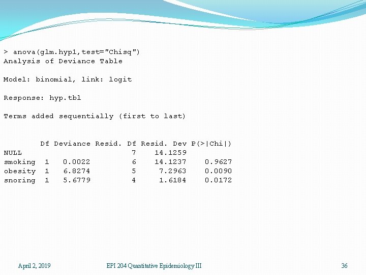
> anova(glm. hyp 1, test="Chisq") Analysis of Deviance Table Model: binomial, link: logit Response: hyp. tbl Terms added sequentially (first to last) Df Deviance Resid. Df Resid. Dev P(>|Chi|) NULL 7 14. 1259 smoking 1 0. 0022 6 14. 1237 0. 9627 obesity 1 6. 8274 5 7. 2963 0. 0090 snoring 1 5. 6779 4 1. 6184 0. 0172 April 2, 2019 EPI 204 Quantitative Epidemiology III 36

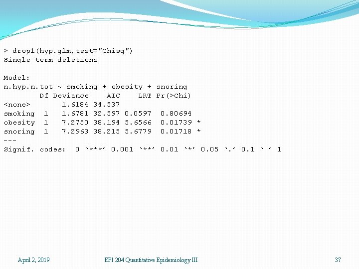
> drop 1(hyp. glm, test="Chisq") Single term deletions Model: n. hyp. n. tot ~ smoking + obesity + snoring Df Deviance AIC LRT Pr(>Chi) <none> 1. 6184 34. 537 smoking 1 1. 6781 32. 597 0. 0597 0. 80694 obesity 1 7. 2750 38. 194 5. 6566 0. 01739 * snoring 1 7. 2963 38. 215 5. 6779 0. 01718 * --Signif. codes: 0 ‘***’ 0. 001 ‘**’ 0. 01 ‘*’ 0. 05 ‘. ’ 0. 1 ‘ ’ 1 April 2, 2019 EPI 204 Quantitative Epidemiology III 37

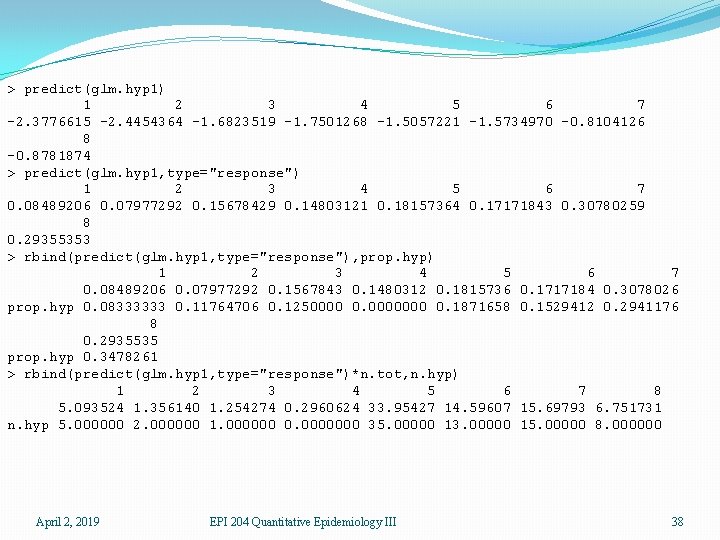
> predict(glm. hyp 1) 1 2 3 4 5 6 7 -2. 3776615 -2. 4454364 -1. 6823519 -1. 7501268 -1. 5057221 -1. 5734970 -0. 8104126 8 -0. 8781874 > predict(glm. hyp 1, type="response") 1 2 3 4 5 6 7 0. 08489206 0. 07977292 0. 15678429 0. 14803121 0. 18157364 0. 17171843 0. 30780259 8 0. 29355353 > rbind(predict(glm. hyp 1, type="response"), prop. hyp) 1 2 3 4 5 6 7 0. 08489206 0. 07977292 0. 1567843 0. 1480312 0. 1815736 0. 1717184 0. 3078026 prop. hyp 0. 08333333 0. 11764706 0. 1250000 0. 0000000 0. 1871658 0. 1529412 0. 2941176 8 0. 2935535 prop. hyp 0. 3478261 > rbind(predict(glm. hyp 1, type="response")*n. tot, n. hyp) 1 2 3 4 5 6 7 8 5. 093524 1. 356140 1. 254274 0. 2960624 33. 95427 14. 59607 15. 69793 6. 751731 n. hyp 5. 000000 2. 000000 1. 000000 0. 0000000 35. 00000 13. 00000 15. 00000 8. 000000 April 2, 2019 EPI 204 Quantitative Epidemiology III 38

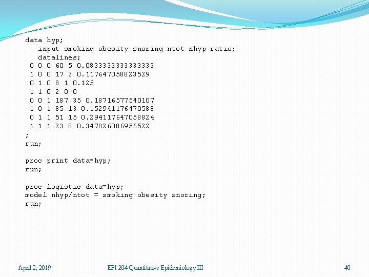
R and SAS Differences �The only difference is caused by R using 0/1 coding for two-level class variables and SAS using -1/1 coding. �So for the SAS code we used numeric 0/1 instead of strings. �The hypothesis tests are essentially the same, as are the predicted values for each category, but the coefficients would differ if we used strings like “Yes” and “No” in SAS. �You can try running the SAS version and compare the results. April 2, 2019 EPI 204 Quantitative Epidemiology III 39

data hyp; input smoking obesity snoring ntot nhyp ratio; datalines; 0 0 0 60 5 0. 083333333 1 0 0 17 2 0. 117647058823529 0 1 0 8 1 0. 125 1 1 0 2 0 0 1 187 35 0. 18716577540107 1 0 1 85 13 0. 152941176470588 0 1 1 51 15 0. 294117647058824 1 1 1 23 8 0. 347826086956522 ; run; proc print data=hyp; run; proc logistic data=hyp; model nhyp/ntot = smoking obesity snoring; run; April 2, 2019 EPI 204 Quantitative Epidemiology III 40

Parameter Intercept smoking obesity snoring Analysis of Maximum Likelihood Estimates Standard Wald DF Estimate Error Chi-Square Pr > Chi. Sq 1 -2. 3776 0. 3802 39. 1119 <. 0001 1 -0. 0678 0. 2781 0. 0594 0. 8075 1 0. 6953 0. 2851 5. 9486 0. 0147 1 0. 8718 0. 3976 4. 8091 0. 0283 Estimate Std. Error z value (Intercept) -2. 37766 0. 38018 -6. 254 smoking. Yes -0. 06777 0. 27812 -0. 244 obesity. Yes 0. 69531 0. 28509 2. 439 snoring. Yes 0. 87194 0. 39757 2. 193 Pr(>|z|) 4 e-10 *** 0. 8075 0. 0147 * 0. 0283 * Wald Chi-Square is the square of the “z-value” The coefficient estimates may be different in SAS depending on the coding (0/1 vs. -1/1) but the p-values should be the same. April 2, 2019 EPI 204 Quantitative Epidemiology III 41

Odds Ratio Estimates Effect smoking obesity snoring Point Estimate 0. 934 2. 004 2. 391 > exp(coef(glm. hyp 2)) (Intercept) smoking. Yes 0. 09276726 0. 93447081 obesity. Yes 2. 00432951 95% Wald Confidence Limits 0. 542 1. 146 1. 097 1. 612 3. 505 5. 212 snoring. Yes 2. 39154432 > exp(confint. default(glm. hyp 2)) 2. 5 % 97. 5 % (Intercept) 0. 04403329 0. 1954377 smoking. Yes 0. 54178381 1. 6117789 obesity. Yes 1. 14631567 3. 5045641 snoring. Yes 1. 09714274 5. 2130721 April 2, 2019 EPI 204 Quantitative Epidemiology III 42

Access to R and SAS �You can download the main R binary at https: //cran. r-project. org/ �R Studio (a integrated environment) is at https: //www. rstudio. com/ �R packages can be installed from within R. In Windows, it is best to install packages after starting R as an administrator �SAS University Edition is free if you have a. edu email address. Start at http: //www. sas. com/en_us/software/universityedition. html or just search for SAS University Edition �Be sure to read the Quick. Start Guide because it installs from within Oracle Virtual. Box. April 2, 2019 EPI 204 Quantitative Epidemiology III 43