Logistic Regression 4 Sociology 8811 Lecture 9 Copyright

Logistic Regression 4 Sociology 8811 Lecture 9 Copyright © 2007 by Evan Schofer Do not copy or distribute without permission

Announcements • Paper # 1 handed out today • Due March 8

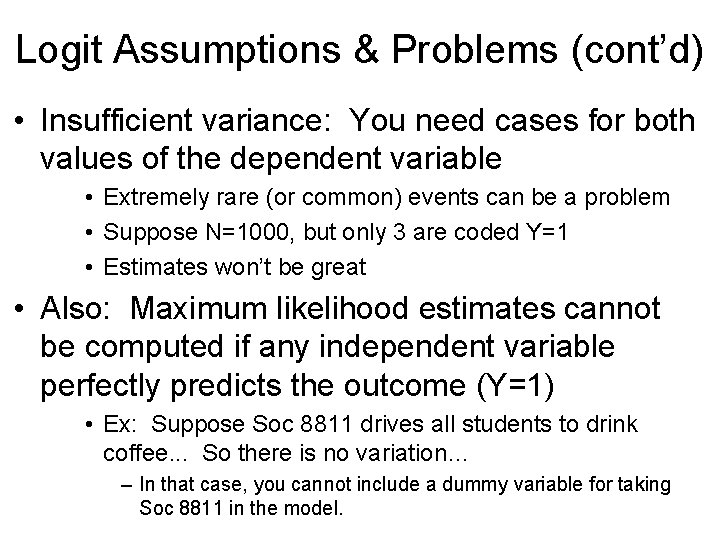
Logit Assumptions & Problems (cont’d) • Insufficient variance: You need cases for both values of the dependent variable • Extremely rare (or common) events can be a problem • Suppose N=1000, but only 3 are coded Y=1 • Estimates won’t be great • Also: Maximum likelihood estimates cannot be computed if any independent variable perfectly predicts the outcome (Y=1) • Ex: Suppose Soc 8811 drives all students to drink coffee. . . So there is no variation… – In that case, you cannot include a dummy variable for taking Soc 8811 in the model.

Logit Assumptions & Problems • Model specification / Omitted variable bias • Just like any regression model, it is critical to include appropriate variables in the model • Omission of important factors or ‘controls’ will lead to misleading results.

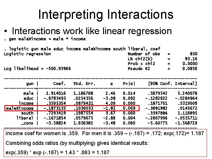
Interpreting Interactions • Interactions work like linear regression. gen male. Xincome = male * income. logistic gun male educ income male. Xincome south liberal, coef Logistic regression Number of obs LR chi 2(6) Prob > chi 2 Log likelihood = -500. 93966 Pseudo R 2 = = 850 93. 10 0. 0000 0. 0850 ---------------------------------------gun | Coef. Std. Err. z P>|z| [95% Conf. Interval] -------+--------------------------------male | 2. 914016 1. 186788 2. 46 0. 014. 5879542 5. 240078 educ | -. 0783493. 0254356 -3. 08 0. 002 -. 1282022 -. 0284964 income |. 3595354. 0879431 4. 09 0. 000. 1871701. 5319008 male. Xincome | -. 1873155. 1030033 -1. 82 0. 069 -. 3891982. 0145672 south |. 7293419. 1987554 3. 67 0. 000. 3397886 1. 118895 liberal | -. 1671854. 0579675 -2. 88 0. 004 -. 2807996 -. 0535711 _cons | -3. 58824 1. 030382 -3. 48 0. 000 -5. 60775 -1. 568729 --------------------------------------- Income coef for women is. 359. For men it is. 359 – (-. 187) =. 172; exp(. 172)= 1. 187 Combining odds ratios (by multiplying) gives identical results: exp(. 359) * exp (-. 187) = 1. 43 *. 083 = 1. 187

Real World Example: Coups • Issue: Many countries face threat of a coup d’etat – violent overthrow of the regime • What factors whether a countries will have a coup? • Paper Handout: Belkin and Schofer (2005) • What are the basic findings? • How much do the odds of a coup differ for military regimes vs. civilian governments? – b=1. 74; (e 1. 74 -1)*100% = +470% • What about a 2 -point increase in log GDP? – b=-. 233; ((e-. 233 * e-. 233) -1)*100% = -37%

Real World Example • Goyette, Kimberly and Yu Xie. 1999. “Educational Expectations of Asian American Youths: Determinants and Ethnic Differences. ” Sociology of Education, 72, 1: 22 -36. • What was the paper about? • • What was the analysis? Dependent variable? Key independent variables? Findings? Issues / comments / criticisms?

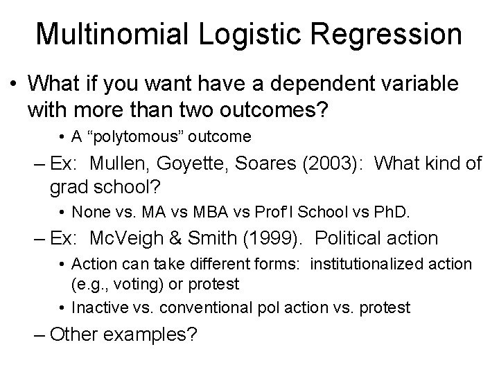
Multinomial Logistic Regression • What if you want have a dependent variable with more than two outcomes? • A “polytomous” outcome – Ex: Mullen, Goyette, Soares (2003): What kind of grad school? • None vs. MA vs MBA vs Prof’l School vs Ph. D. – Ex: Mc. Veigh & Smith (1999). Political action • Action can take different forms: institutionalized action (e. g. , voting) or protest • Inactive vs. conventional pol action vs. protest – Other examples?

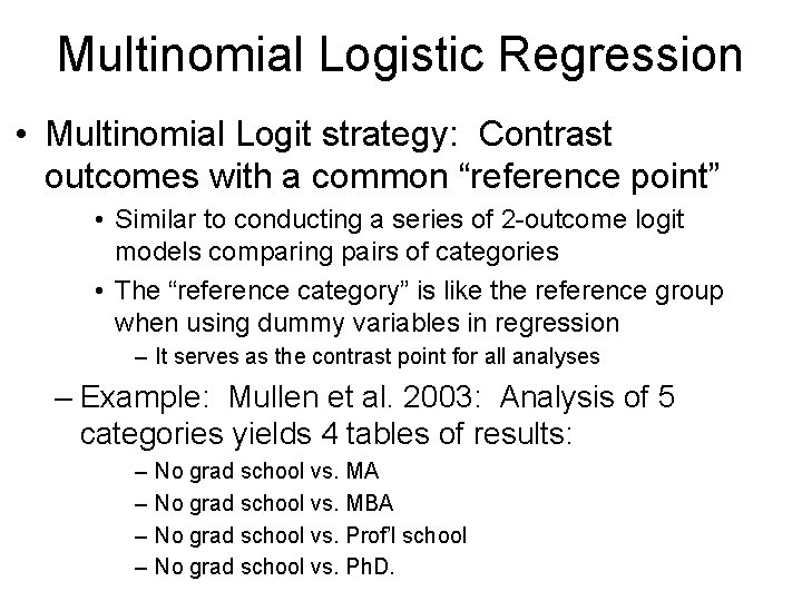
Multinomial Logistic Regression • Multinomial Logit strategy: Contrast outcomes with a common “reference point” • Similar to conducting a series of 2 -outcome logit models comparing pairs of categories • The “reference category” is like the reference group when using dummy variables in regression – It serves as the contrast point for all analyses – Example: Mullen et al. 2003: Analysis of 5 categories yields 4 tables of results: – – No grad school vs. MA No grad school vs. MBA No grad school vs. Prof’l school No grad school vs. Ph. D.

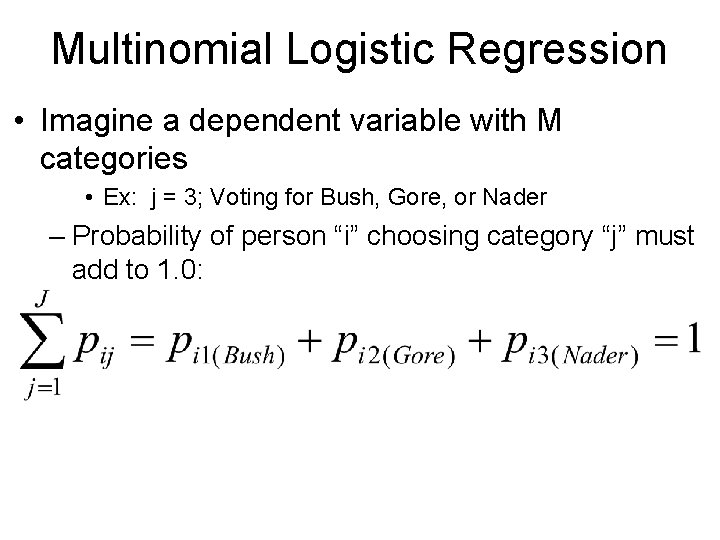
Multinomial Logistic Regression • Imagine a dependent variable with M categories • Ex: j = 3; Voting for Bush, Gore, or Nader – Probability of person “i” choosing category “j” must add to 1. 0:

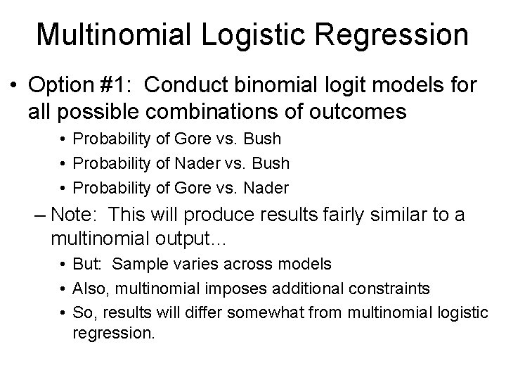
Multinomial Logistic Regression • Option #1: Conduct binomial logit models for all possible combinations of outcomes • Probability of Gore vs. Bush • Probability of Nader vs. Bush • Probability of Gore vs. Nader – Note: This will produce results fairly similar to a multinomial output… • But: Sample varies across models • Also, multinomial imposes additional constraints • So, results will differ somewhat from multinomial logistic regression.

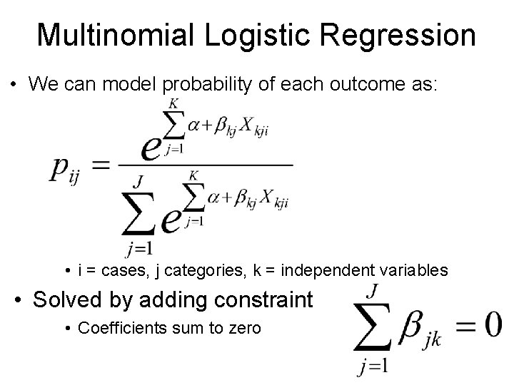
Multinomial Logistic Regression • We can model probability of each outcome as: • i = cases, j categories, k = independent variables • Solved by adding constraint • Coefficients sum to zero

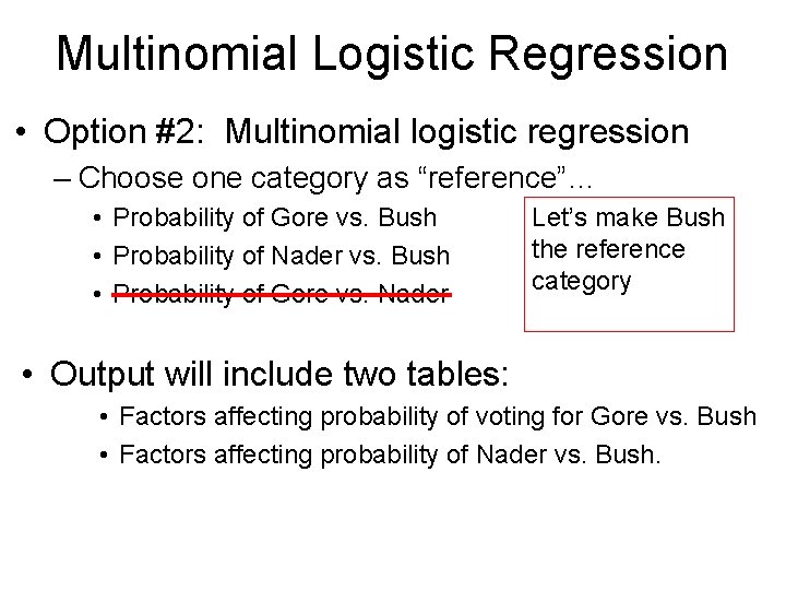
Multinomial Logistic Regression • Option #2: Multinomial logistic regression – Choose one category as “reference”… • Probability of Gore vs. Bush • Probability of Nader vs. Bush • Probability of Gore vs. Nader Let’s make Bush the reference category • Output will include two tables: • Factors affecting probability of voting for Gore vs. Bush • Factors affecting probability of Nader vs. Bush.

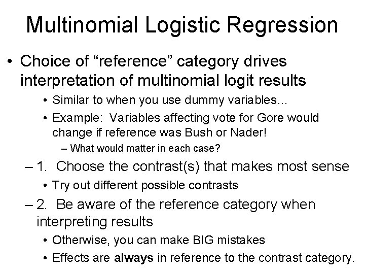
Multinomial Logistic Regression • Choice of “reference” category drives interpretation of multinomial logit results • Similar to when you use dummy variables… • Example: Variables affecting vote for Gore would change if reference was Bush or Nader! – What would matter in each case? – 1. Choose the contrast(s) that makes most sense • Try out different possible contrasts – 2. Be aware of the reference category when interpreting results • Otherwise, you can make BIG mistakes • Effects are always in reference to the contrast category.

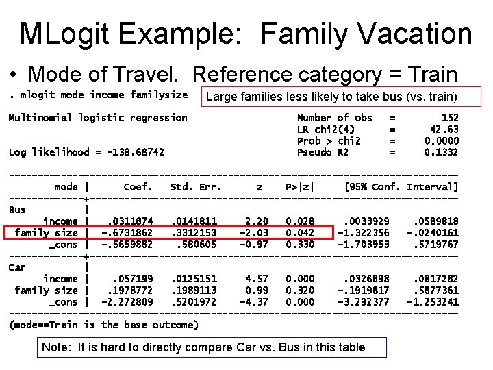
MLogit Example: Family Vacation • Mode of Travel. Reference category = Train. mlogit mode income familysize Multinomial logistic regression Log likelihood = -138. 68742 Large families less likely to take bus (vs. train) Number of obs LR chi 2(4) Prob > chi 2 Pseudo R 2 = = 152 42. 63 0. 0000 0. 1332 ---------------------------------------mode | Coef. Std. Err. z P>|z| [95% Conf. Interval] -------+--------------------------------Bus | income |. 0311874. 0141811 2. 20 0. 028. 0033929. 0589818 family size | -. 6731862. 3312153 -2. 03 0. 042 -1. 322356 -. 0240161 _cons | -. 5659882. 580605 -0. 97 0. 330 -1. 703953. 5719767 -------+--------------------------------Car | income |. 057199. 0125151 4. 57 0. 000. 0326698. 0817282 family size |. 1978772. 1989113 0. 99 0. 320 -. 1919817. 5877361 _cons | -2. 272809. 5201972 -4. 37 0. 000 -3. 292377 -1. 253241 ---------------------------------------(mode==Train is the base outcome) Note: It is hard to directly compare Car vs. Bus in this table

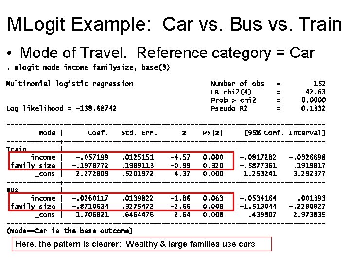
MLogit Example: Car vs. Bus vs. Train • Mode of Travel. Reference category = Car. mlogit mode income familysize, base(3) Multinomial logistic regression Log likelihood = -138. 68742 Number of obs LR chi 2(4) Prob > chi 2 Pseudo R 2 = = 152 42. 63 0. 0000 0. 1332 ---------------------------------------mode | Coef. Std. Err. z P>|z| [95% Conf. Interval] -------+--------------------------------Train | income | -. 057199. 0125151 -4. 57 0. 000 -. 0817282 -. 0326698 family size | -. 1978772. 1989113 -0. 99 0. 320 -. 5877361. 1919817 _cons | 2. 272809. 5201972 4. 37 0. 000 1. 253241 3. 292377 -------+--------------------------------Bus | income | -. 0260117. 0139822 -1. 86 0. 063 -. 0534164. 001393 family size | -. 8710634. 3275472 -2. 66 0. 008 -1. 513044 -. 2290827 _cons | 1. 706821. 6464476 2. 64 0. 008. 439807 2. 973835 ---------------------------------------(mode==Car is the base outcome) Here, the pattern is clearer: Wealthy & large families use cars

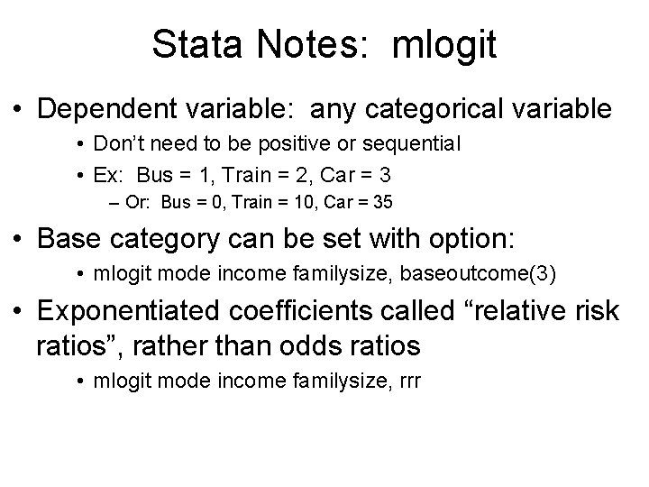
Stata Notes: mlogit • Dependent variable: any categorical variable • Don’t need to be positive or sequential • Ex: Bus = 1, Train = 2, Car = 3 – Or: Bus = 0, Train = 10, Car = 35 • Base category can be set with option: • mlogit mode income familysize, baseoutcome(3) • Exponentiated coefficients called “relative risk ratios”, rather than odds ratios • mlogit mode income familysize, rrr

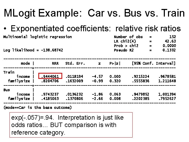
MLogit Example: Car vs. Bus vs. Train • Exponentiated coefficients: relative risk ratios Multinomial logistic regression Log likelihood = -138. 68742 Number of obs LR chi 2(4) Prob > chi 2 Pseudo R 2 = = 152 42. 63 0. 0000 0. 1332 ---------------------------------------mode | RRR Std. Err. z P>|z| [95% Conf. Interval] -------+--------------------------------Train | income |. 9444061. 0118194 -4. 57 0. 000. 9215224. 9678581 familysize |. 8204706. 1632009 -0. 99 0. 320. 5555836 1. 211648 -------+--------------------------------Bus | income |. 9743237. 0136232 -1. 86 0. 063. 9479852 1. 001394 familysize |. 4185063. 1370806 -2. 66 0. 008. 2202385. 7952627 ---------------------------------------(mode==Car is the base outcome) exp(-. 057)=. 94. Interpretation is just like odds ratios… BUT comparison is with reference category.

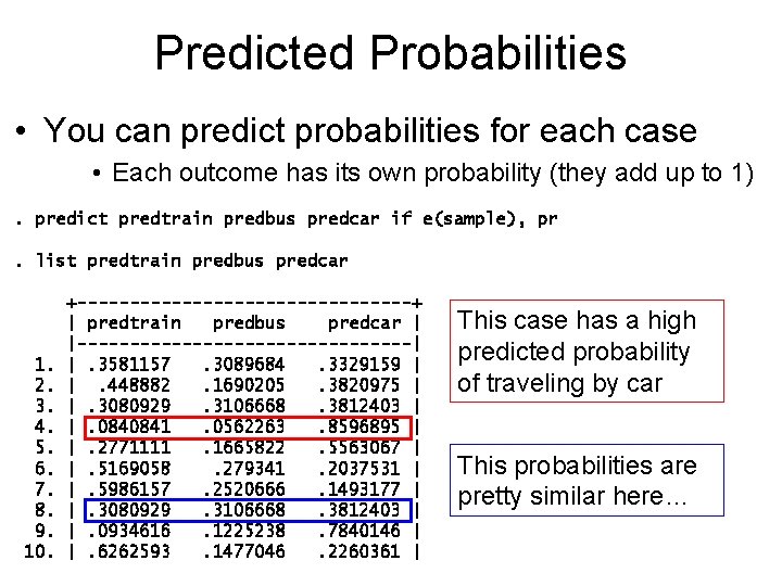
Predicted Probabilities • You can predict probabilities for each case • Each outcome has its own probability (they add up to 1). predict predtrain predbus predcar if e(sample), pr. list predtrain predbus predcar 1. 2. 3. 4. 5. 6. 7. 8. 9. 10. +----------------+ | predtrain predbus predcar | |----------------| |. 3581157. 3089684. 3329159 | |. 448882. 1690205. 3820975 | |. 3080929. 3106668. 3812403 | |. 0840841. 0562263. 8596895 | |. 2771111. 1665822. 5563067 | |. 5169058. 279341. 2037531 | |. 5986157. 2520666. 1493177 | |. 3080929. 3106668. 3812403 | |. 0934616. 1225238. 7840146 | |. 6262593. 1477046. 2260361 | This case has a high predicted probability of traveling by car This probabilities are pretty similar here…

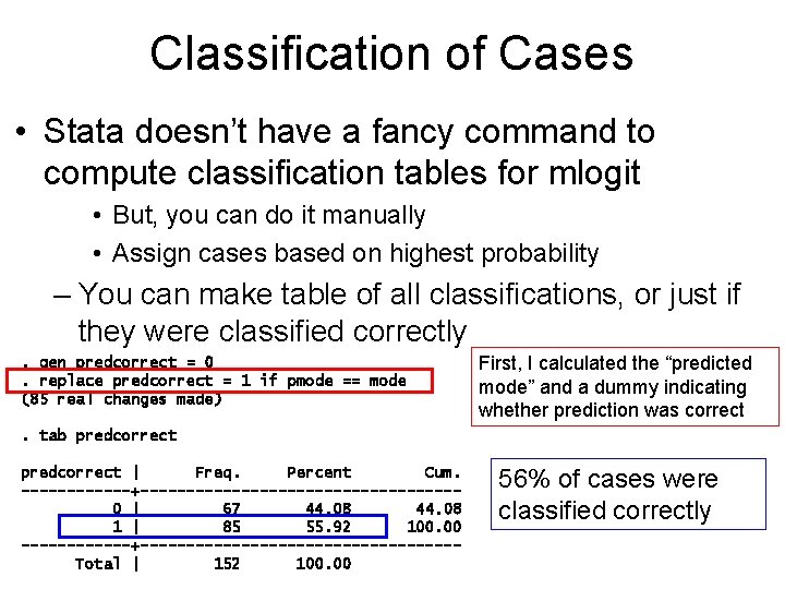
Classification of Cases • Stata doesn’t have a fancy command to compute classification tables for mlogit • But, you can do it manually • Assign cases based on highest probability – You can make table of all classifications, or just if they were classified correctly. gen predcorrect = 0. replace predcorrect = 1 if pmode == mode (85 real changes made) First, I calculated the “predicted mode” and a dummy indicating whether prediction was correct . tab predcorrect | Freq. Percent Cum. ------+-----------------0 | 67 44. 08 1 | 85 55. 92 100. 00 ------+-----------------Total | 152 100. 00 56% of cases were classified correctly

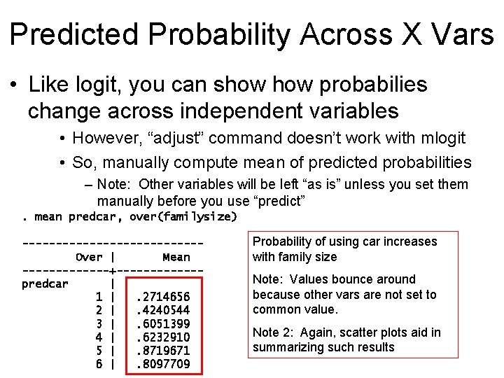
Predicted Probability Across X Vars • Like logit, you can show probabilies change across independent variables • However, “adjust” command doesn’t work with mlogit • So, manually compute mean of predicted probabilities – Note: Other variables will be left “as is” unless you set them manually before you use “predict”. mean predcar, over(familysize) -------------Over | Mean -------+------predcar | 1 |. 2714656 2 |. 4240544 3 |. 6051399 4 |. 6232910 5 |. 8719671 6 |. 8097709 Probability of using car increases with family size Note: Values bounce around because other vars are not set to common value. Note 2: Again, scatter plots aid in summarizing such results

Stata Notes: mlogit • Like logit, you can’t include variables that perfectly predict the outcome • Note: Stata “logit” command gives a warning of this • mlogit command doesn’t give a warning, but coefficient will have z-value of zero, p-value =1 • Remove problematic variables if this occurs!

Hypothesis Tests • Individual coefficients can be tested as usual • Wald test/z-values provided for each variable • However, adding a new variable to model actually yields more than one coefficient • If you have 4 categories, you’ll get 3 coefficients • LR tests are especially useful because you can test for improved fit across the whole model

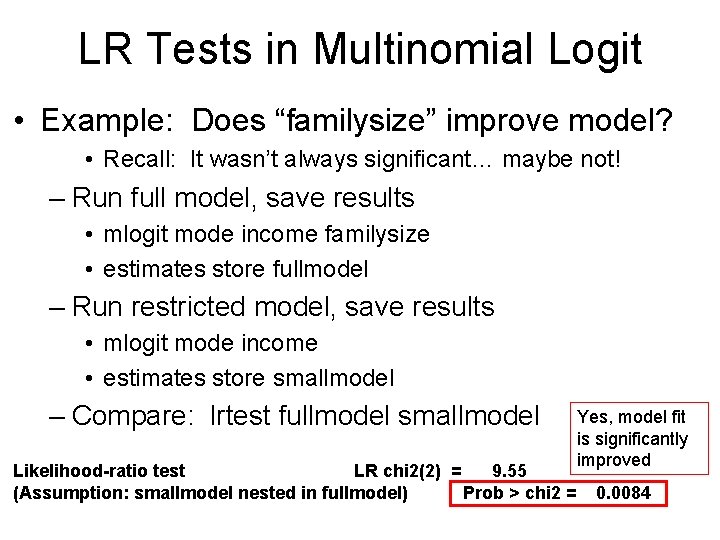
LR Tests in Multinomial Logit • Example: Does “familysize” improve model? • Recall: It wasn’t always significant… maybe not! – Run full model, save results • mlogit mode income familysize • estimates store fullmodel – Run restricted model, save results • mlogit mode income • estimates store smallmodel – Compare: lrtest fullmodel smallmodel Likelihood-ratio test LR chi 2(2) = 9. 55 (Assumption: smallmodel nested in fullmodel) Prob > chi 2 = Yes, model fit is significantly improved 0. 0084

Multinomial Logit Assumptions: IIA • Multinomial logit is designed for outcomes that are not complexly interrelated • Critical assumption: Independence of Irrelevant Alternatives (IIA) • Odds of one outcome versus another should be independent of other alternatives – Problems often come up when dealing with individual choices… • Multinomial logit is not appropriate if the assumption is violated.

Multinomial Logit Assumptions: IIA • IIA Assumption Example: – Odds of voting for Gore vs. Bush should not change if Nader is added or removed from ballot • If Nader is removed, those voters should choose Bush & Gore in similar pattern to rest of sample – Is IIA assumption likely met in election model? – NO! If Nader were removed, those voters would likely vote for Gore • Removal of Nader would change odds ratio for Bush/Gore.

Multinomial Logit Assumptions: IIA • IIA Example 2: Consumer Preferences – Options: coffee, Gatorade, Coke • Might meet IIA assumption – Options: coffee, Gatorade, Coke, Pepsi • Won’t meet IIA assumption. Coke & Pepsi are very similar – substitutable. • Removal of Pepsi will drastically change odds ratios for coke vs. others.

Multinomial Logit Assumptions: IIA • Solution: Choose categories carefully when doing multinomial logit! • Long and Freese (2006), quoting Mcfadden: • “Multinomial and conditional logit models should only be used in cases where the alternatives “can plausibly be assumed to be distinct and weighed independently in the eyes of the decisionmaker. ” • Categories should be “distinct alternatives”, not substitutes – Note: There are some formal tests for violation of IIA. But they don’t work well. Don’t use them. • See Long and Freese (2006) p. 243

Multinomial Assumptions/Problems • Aside from IIA, assumptions & problems of multinomial logit are similar to standard logit • Sample size – You often want to estimate MANY coefficients, so watch out for small N • • Outliers Multicollinearity Model specification / omitted variable bias Etc.

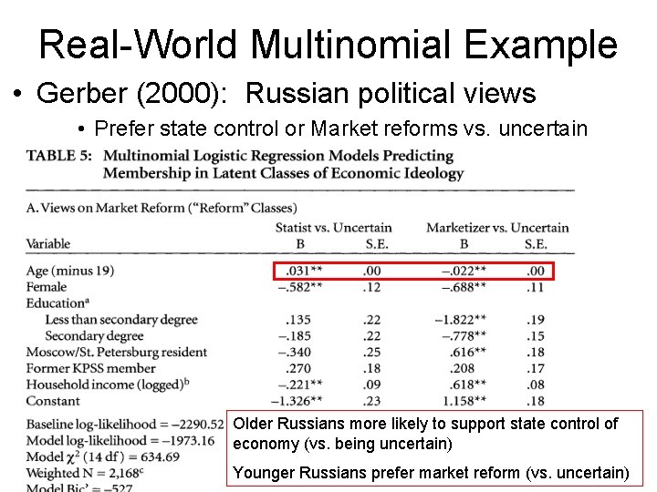
Real-World Multinomial Example • Gerber (2000): Russian political views • Prefer state control or Market reforms vs. uncertain Older Russians more likely to support state control of economy (vs. being uncertain) Younger Russians prefer market reform (vs. uncertain)

Other Logit-type Models • Ordered logit: Appropriate for ordered categories • Useful for non-interval measures • Useful if there are too few categories to use OLS • Conditional Logit • Useful for “alternative specific” data – Ex: Data on characteristics of voters AND candidates • Problems with IIA assumption • Nested logit • Alternative specific multinomial probit • And others!