Logistic Regression Geoff Hulten Overview of Logistic Regression

Logistic Regression Geoff Hulten

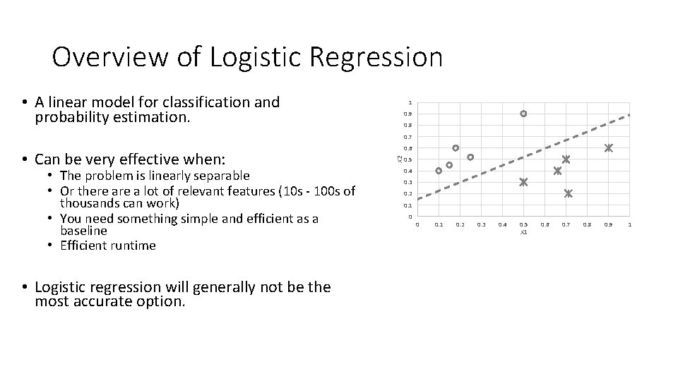
Overview of Logistic Regression • A linear model for classification and probability estimation. 1 0. 9 0. 8 0. 7 • The problem is linearly separable • Or there a lot of relevant features (10 s - 100 s of thousands can work) • You need something simple and efficient as a baseline • Efficient runtime • Logistic regression will generally not be the most accurate option. X 2 • Can be very effective when: 0. 6 0. 5 0. 4 0. 3 0. 2 0. 1 0 0 0. 1 0. 2 0. 3 0. 4 0. 5 X 1 0. 6 0. 7 0. 8 0. 9 1

Components of Learning Algorithm: Logistic Regression • Model Structure – Linear model with sigmoid activation • Loss Function – Log Loss • Optimization Method – Gradient Descent

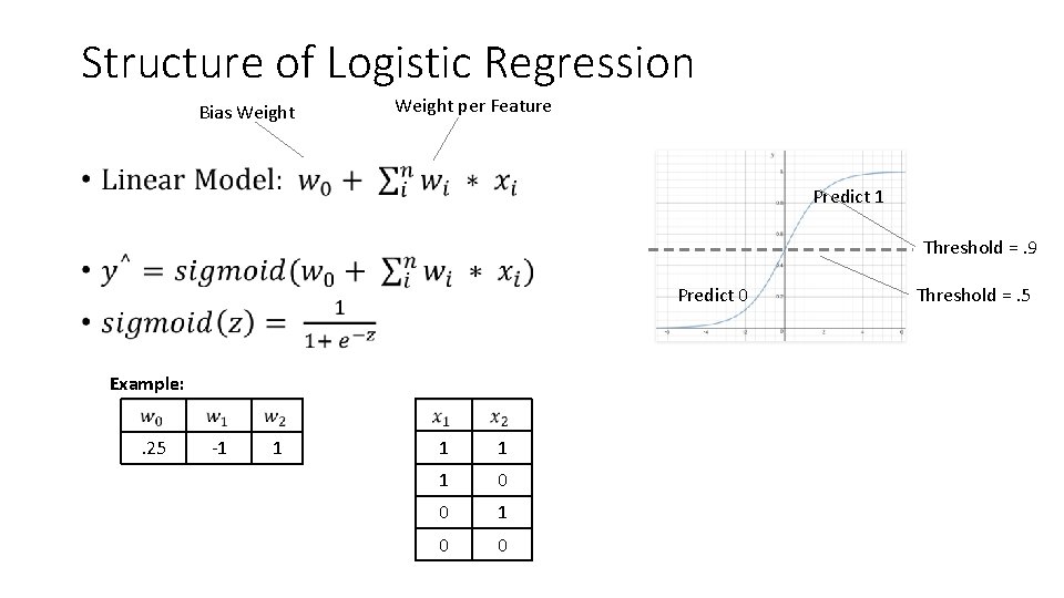
Structure of Logistic Regression Bias Weight per Feature • Predict 1 Threshold =. 9 Predict 0 Example: . 25 -1 1 1 0 0 Threshold =. 5

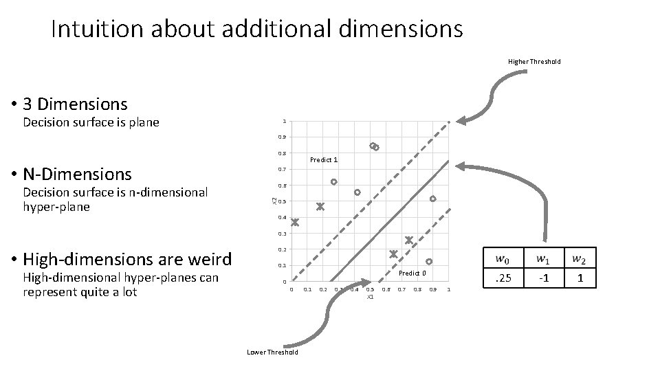
Intuition about additional dimensions Higher Threshold • 3 Dimensions Decision surface is plane 1 0. 9 0. 8 • N-Dimensions 0. 7 0. 6 X 2 Decision surface is n-dimensional hyper-plane Predict 1 0. 5 0. 4 0. 3 • High-dimensions are weird High-dimensional hyper-planes can represent quite a lot 0. 2 0. 1 0 Predict 0 0 Lower Threshold 0. 1 0. 2 0. 3 0. 4 0. 5 X 1 0. 6 0. 7 0. 8 . 25 0. 9 1 -1 1

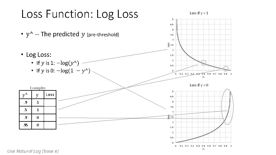
Loss Function: Log Loss if y = 1 5 4 • 3. 5 Loss 3 2. 5 2 1. 5 1 0. 5 0 0 0. 1 0. 2 0. 3 0. 4 0. 5 0. 6 0. 7 0. 8 0. 9 Y^ 1 Loss if y = 0 Examples 5 Loss 1 . 105 . 5 1 . 693 . 9 0 2. 3 . 95 0 2. 99 4 3. 5 3 Loss . 9 4. 5 2 1. 5 1 0. 5 0 Use Natural Log (base e) 0 0. 1 0. 2 0. 3 0. 4 0. 5 0. 6 0. 7 0. 8 0. 9 Y^ 1

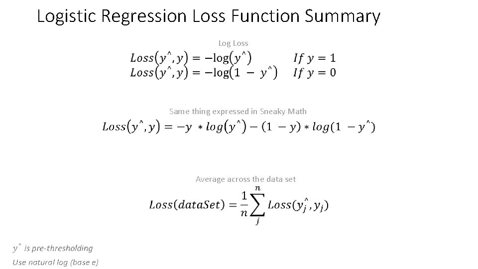
Logistic Regression Loss Function Summary Log Loss • Same thing expressed in Sneaky Math Average across the data set Use natural log (base e)

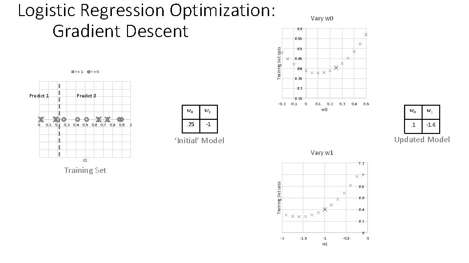
Logistic Regression Optimization: Gradient Descent 6. 6 6. 55 Training Set Loss Y = 1 Vary w 0 Y = 0 6. 5 6. 4 6. 35 6. 3 Predict 1 Predict 0 -0. 2 0. 1 0. 2 0. 3 0. 4 0. 5 0. 6 0. 7 0. 8 0. 9 1 . 25 0. 1 w 0 0. 2 0. 3 0. 4 0. 5 -1 . 1 -1. 6 Updated Model ‘Initial’ Model Vary w 1 X 1 7. 2 Training Set 7 Training Set Loss 0 6. 25 -0. 1 0 6. 8 6. 6 6. 4 6. 2 -2 -1. 5 -1 w 1 -0. 5 6 0

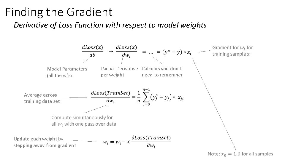
Finding the Gradient Derivative of Loss Function with respect to model weights Partial Derivative Calculus you don’t per weight need to remember Model Parameters (all the w’s) Average across training data set Update each weight by stepping away from gradient •

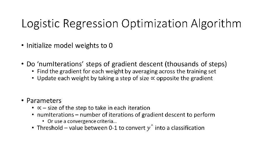
Logistic Regression Optimization Algorithm •