March 2007 doc IEEE 802 15 070559 r

March 2007 doc. : IEEE 802. 15 -07/0559 r 3 Project: IEEE P 802. 15 Working Group for Wireless Personal Area Networks (WPANs) Submission Title: [CM MATLAB Release Support Document] Date Submitted: [March 13 2007] Source: [Hiroshi Harada, Ryuhei Funada, Hirokazu Sawada, Shuzo Kato ] Company [NICT], E-Mail: [harada@nict. go. jp, funada@nict. go. jp, sawahiro@nict. go. jp, shu. kato@nict. go. jp] Source: [Rick Roberts] Company [Intel, Corp], E-Mail: [richard. d. roberts@intel. com] Re: [] Abstract: [This document supports the Matlab CM code 15 -07/648 r 0. ] Purpose: [] Notice: This document has been prepared to assist the IEEE P 802. 15. It is offered as a basis for discussion and is not binding on the contributing individual(s) or organization(s). The material in this document is subject to change in form and content after further study. The contributor(s) reserve(s) the right to add, amend or withdraw material contained herein. Release: The contributor acknowledges and accepts that this contribution becomes the property of IEEE and may be made publicly available by P 802. 15. Submission Slide 1 Hiroshi Harada (NICT), Rick Roberts (Intel)

March 2007 doc. : IEEE 802. 15 -07/0559 r 3 This document “documents” the MATLAB CM code 15 -07/648 r 0. Submission Slide 2 Hiroshi Harada (NICT), Rick Roberts (Intel)

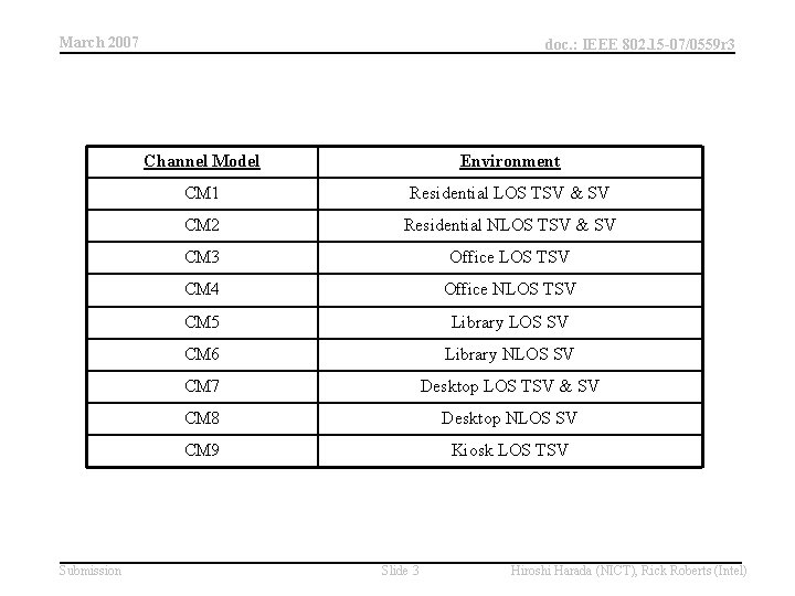
March 2007 Submission doc. : IEEE 802. 15 -07/0559 r 3 Channel Model Environment CM 1 Residential LOS TSV & SV CM 2 Residential NLOS TSV & SV CM 3 Office LOS TSV CM 4 Office NLOS TSV CM 5 Library LOS SV CM 6 Library NLOS SV CM 7 Desktop LOS TSV & SV CM 8 Desktop NLOS SV CM 9 Kiosk LOS TSV Slide 3 Hiroshi Harada (NICT), Rick Roberts (Intel)

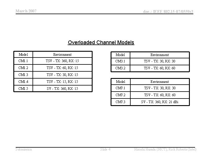
March 2007 doc. : IEEE 802. 15 -07/0559 r 3 Overloaded Channel Models Model Environment CM 1. 1 TSV - TX: 360, RX: 15 CM 3. 1 TSV - TX: 30, RX: 30 CM 1. 2 TSV - TX: 60, RX: 15 CM 3. 2 TSV - TX: 60, RX: 60 CM 1. 3 TSV - TX: 30, RX: 15 CM 1. 4 TSV - TX: 15, RX: 15 Model Environment CM 1. 5 SV - TX: 360, RX: 15 CM 7. 1 TSV - TX: 30, RX: 30 CM 7. 2 TSV - TX: 60, RX: 60 CM 7. 3 SV - TX: 360, RX: 21 d. Bi Submission Slide 4 Hiroshi Harada (NICT), Rick Roberts (Intel)

March 2007 doc. : IEEE 802. 15 -07/0559 r 3 Pertinent Definitions source: 15 -06 -0400 -01 -003 c Submission Slide 5 Hiroshi Harada (NICT), Rick Roberts (Intel)

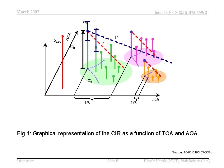
March 2007 doc. : IEEE 802. 15 -07/0559 r 3 1 A 2 G Ao LOS g W 0 1/L 1/l To. A Fig 1: Graphical representation of the CIR as a function of TOA and AOA. Source: 15 -06 -0195 -03 -003 c Submission Slide 6 Hiroshi Harada (NICT), Rick Roberts (Intel)

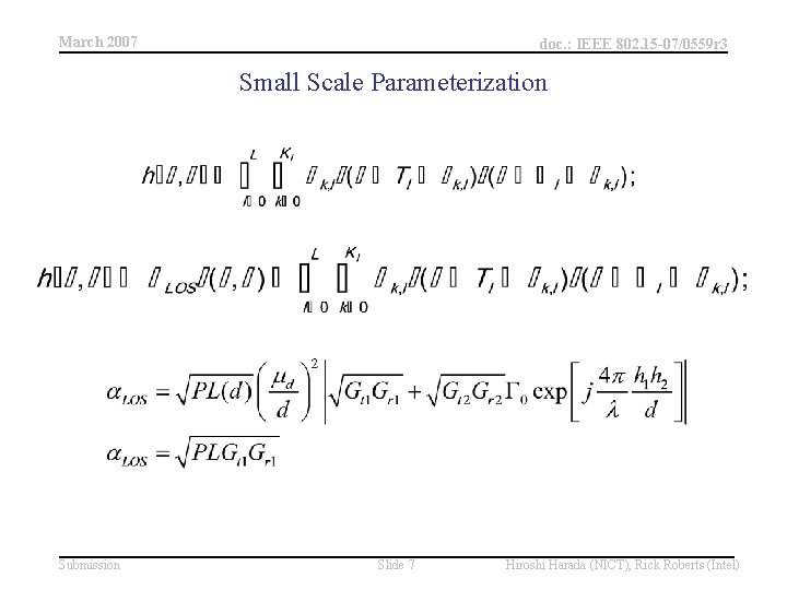
March 2007 doc. : IEEE 802. 15 -07/0559 r 3 Small Scale Parameterization Submission Slide 7 Hiroshi Harada (NICT), Rick Roberts (Intel)

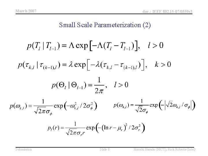
March 2007 doc. : IEEE 802. 15 -07/0559 r 3 Small Scale Parameterization (2) Submission Slide 8 Hiroshi Harada (NICT), Rick Roberts (Intel)

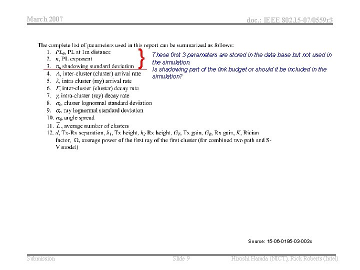
March 2007 doc. : IEEE 802. 15 -07/0559 r 3 } These first 3 parameters are stored in the data base but not used in the simulation. Is shadowing part of the link budget or should it be included in the simulation? Source: 15 -06 -0195 -03 -003 c Submission Slide 9 Hiroshi Harada (NICT), Rick Roberts (Intel)

March 2007 doc. : IEEE 802. 15 -07/0559 r 3 Configuration of the code Submission Slide 10 Hiroshi Harada (NICT), Rick Roberts (Intel)

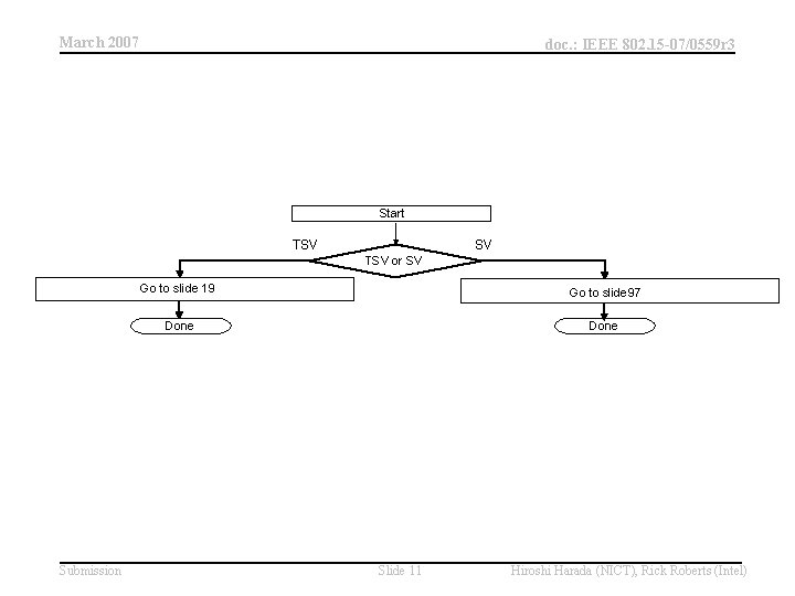
March 2007 doc. : IEEE 802. 15 -07/0559 r 3 Start TSV SV TSV or SV Submission Go to slide 19 Go to slide 97 Done Slide 11 Hiroshi Harada (NICT), Rick Roberts (Intel)

March 2007 doc. : IEEE 802. 15 -07/0559 r 3 TSV Code Support Submission Slide 12 Hiroshi Harada (NICT), Rick Roberts (Intel)

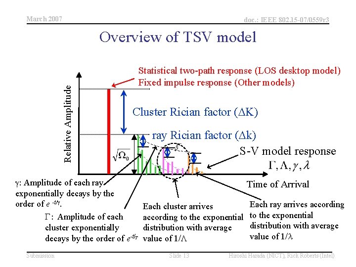
March 2007 doc. : IEEE 802. 15 -07/0559 r 3 Relative Amplitude Overview of TSV model Statistical two-path response (LOS desktop model) Fixed impulse response (Other models) Cluster Rician factor ( K) g: Amplitude of each ray exponentially decays by the order of e -t/g. G： Amplitude of each cluster exponentially decays by the order of e-t/G Submission ray Rician factor ( k) S-V model response Time of Arrival Each cluster arrives according to the exponential distribution with average value of 1/L Slide 13 Each ray arrives according to the exponential distribution with average value of 1/l Hiroshi Harada (NICT), Rick Roberts (Intel)

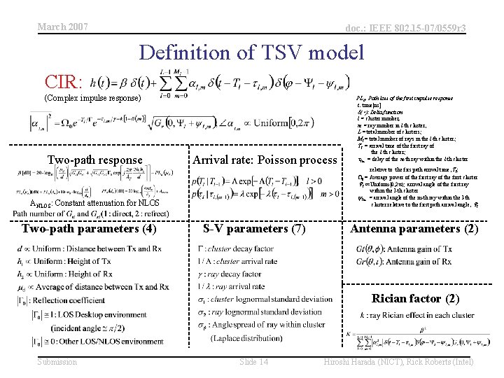
March 2007 doc. : IEEE 802. 15 -07/0559 r 3 Definition of TSV model CIR: (Complex impulse response) Two-path response Arrival rate: Poisson process ANLOS: Constant attenuation for NLOS Two-path parameters (4) S-V parameters (7) PLd: Path loss of the first impulse response t: time[ns] d(・): Delta function l = cluster number, m = ray number in l-th cluster, L = total number of clusters; Ml = total number of rays in the l-th cluster; Tl = arrival time of the first ray of the l-th cluster; l, m = delay of the m-th ray within the l-th cluster relative to the firs path arrival time, Tl; W 0 = Average power of the first ray of the first cluster Yl ∝Uniform[0, 2 p); arrival angle of the first ray within the l-th cluster yl, m = arrival angle of the m-th ray within the l-th cluster relative to the first path arrival angle, Yl Antenna parameters (2) Rician factor (2) Submission Slide 14 Hiroshi Harada (NICT), Rick Roberts (Intel)

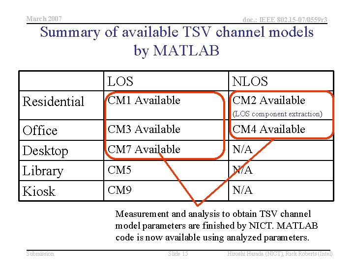
March 2007 doc. : IEEE 802. 15 -07/0559 r 3 Summary of available TSV channel models by MATLAB Residential LOS NLOS CM 1 Available CM 2 Available (LOS component extraction) Office Desktop Library Kiosk CM 3 Available CM 4 Available CM 7 Available N/A CM 5 N/A CM 9 N/A Measurement and analysis to obtain TSV channel model parameters are finished by NICT. MATLAB code is now available using analyzed parameters. Submission Slide 15 Hiroshi Harada (NICT), Rick Roberts (Intel)

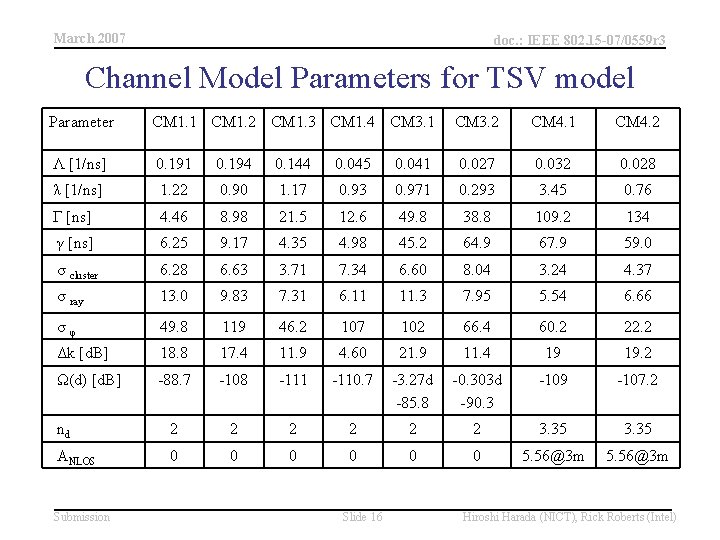
March 2007 doc. : IEEE 802. 15 -07/0559 r 3 Channel Model Parameters for TSV model Parameter CM 1. 1 CM 1. 2 CM 1. 3 CM 1. 4 CM 3. 1 CM 3. 2 CM 4. 1 CM 4. 2 Λ [1/ns] 0. 191 0. 194 0. 144 0. 045 0. 041 0. 027 0. 032 0. 028 λ [1/ns] 1. 22 0. 90 1. 17 0. 93 0. 971 0. 293 3. 45 0. 76 Γ [ns] 4. 46 8. 98 21. 5 12. 6 49. 8 38. 8 109. 2 134 γ [ns] 6. 25 9. 17 4. 35 4. 98 45. 2 64. 9 67. 9 59. 0 σ cluster 6. 28 6. 63 3. 71 7. 34 6. 60 8. 04 3. 24 4. 37 σ ray 13. 0 9. 83 7. 31 6. 11 11. 3 7. 95 5. 54 6. 66 σφ 49. 8 119 46. 2 107 102 66. 4 60. 2 22. 2 Δk [d. B] 18. 8 17. 4 11. 9 4. 60 21. 9 11. 4 19 19. 2 Ω(d) [d. B] -88. 7 -108 -111 -110. 7 -3. 27 d -85. 8 -0. 303 d -90. 3 -109 -107. 2 nd 2 2 2 3. 35 ANLOS 0 0 0 5. 56@3 m Submission Slide 16 Hiroshi Harada (NICT), Rick Roberts (Intel)

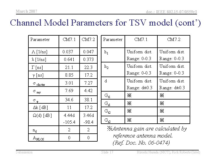
March 2007 doc. : IEEE 802. 15 -07/0559 r 3 Channel Model Parameters for TSV model (cont’) Parameter CM 7. 1 CM 7. 2 Parameter Λ [1/ns] 0. 037　 0. 047 h 1 λ [1/ns] 0. 641 0. 373 Uniform dist. Range: 0 -0. 3 Γ [ns] 21. 1 22. 3 h 2 γ [ns] 8. 85 17. 2 Uniform dist. Range: 0 -0. 3 σ cluster 3. 01 7. 27 d σ ray 7. 69 4. 42 Uniform dist. Range: d± 0. 3 σφ 34. 6 38. 1 Gt 1 ※ ※ 11 17. 2 Gr 1 ※ ※ 4. 44 d -105. 4 3. 46 d -98. 4 Gt 2 ※ ※ Gr 2 ※ ※ nd 2 2 ANLOS 0 0 Δk [d. B] Ω(d) [d. B] Submission CM 7. 1 CM 7. 2 ※Antenna gain are calculated by reference antenna model. (Ref. Doc. No. 06 -0474) Slide 17 Hiroshi Harada (NICT), Rick Roberts (Intel)

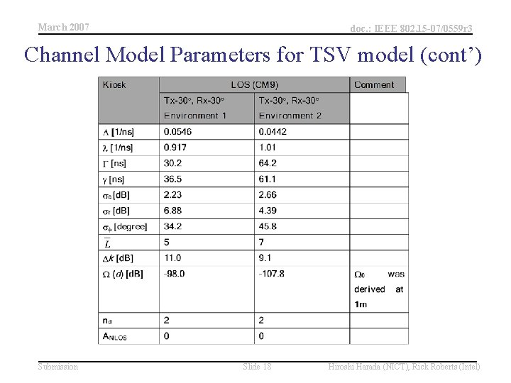
March 2007 doc. : IEEE 802. 15 -07/0559 r 3 Channel Model Parameters for TSV model (cont’) Submission Slide 18 Hiroshi Harada (NICT), Rick Roberts (Intel)

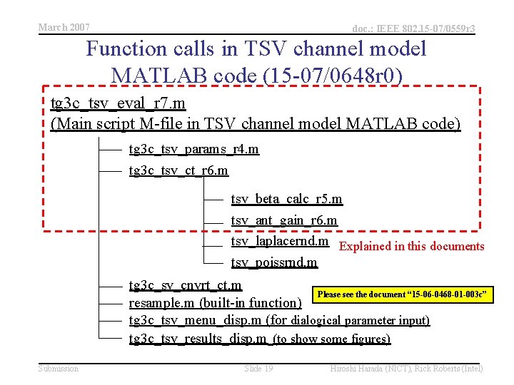
March 2007 doc. : IEEE 802. 15 -07/0559 r 3 Function calls in TSV channel model MATLAB code (15 -07/0648 r 0) tg 3 c_tsv_eval_r 7. m (Main script M-file in TSV channel model MATLAB code) tg 3 c_tsv_params_r 4. m tg 3 c_tsv_ct_r 6. m tsv_beta_calc_r 5. m tsv_ant_gain_r 6. m tsv_laplacernd. m Explained in this documents tsv_poissrnd. m tg 3 c_sv_cnvrt_ct. m Please see the document “ 15 -06 -0468 -01 -003 c” resample. m (built-in function) tg 3 c_tsv_menu_disp. m (for dialogical parameter input) tg 3 c_tsv_results_disp. m (to show some figures) Submission Slide 19 Hiroshi Harada (NICT), Rick Roberts (Intel)

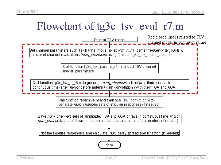
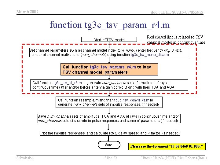
March 2007 doc. : IEEE 802. 15 -07/0559 r 3 Flowchart of tg 3 c_tsv_eval_r 7. m Start of TSV model Red closed line is related to TSV channel model in continuous time Set channel parameters such as channel model index (cm_num), center frequency (fc 0 [GHz]), number of channel realizations (num_channels) using function tg 3 c_tsv_menu_disp. m Call function tg 3 c_tsv_params_r 4. m to load TSV channel model parameters Call function tg 3 c_tsv_ct_r 6. m to generate num_channels sets of amplitude of rays in continuous time (after and/or before antenna gain convolution ) with their TOA and AOA Call function resample. m and then tg 3 c_tsv_convrt_ct. m to generate num_channels sets of impulse responses (if needed) Save num_channels sets of amplitude, TOA and AOA of rays in continuous time and/or num_channels sets of discrete impulse responses and some of parameters (if needed) Plot the impulse responses, and calculate RMS delay spread and K factor (if needed) done Submission Slide 20 Hiroshi Harada (NICT), Rick Roberts (Intel)

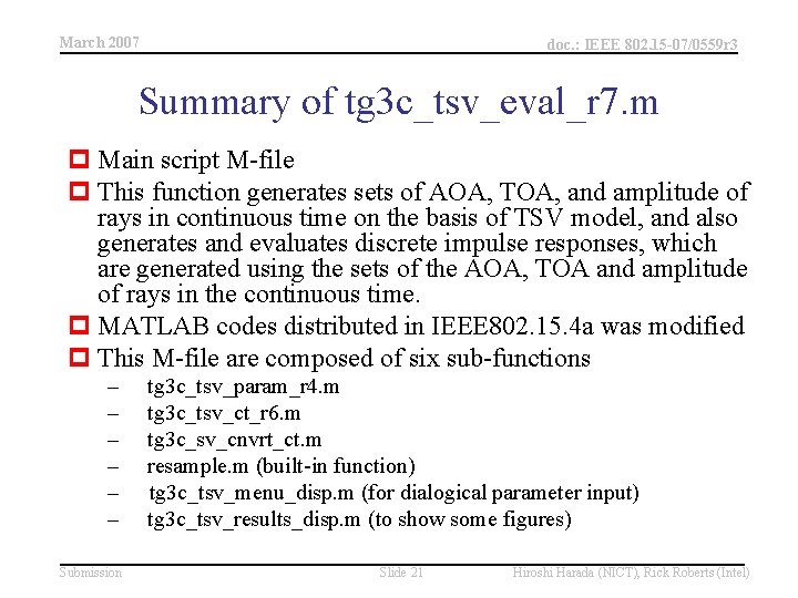
March 2007 doc. : IEEE 802. 15 -07/0559 r 3 Summary of tg 3 c_tsv_eval_r 7. m p Main script M-file p This function generates sets of AOA, TOA, and amplitude of rays in continuous time on the basis of TSV model, and also generates and evaluates discrete impulse responses, which are generated using the sets of the AOA, TOA and amplitude of rays in the continuous time. p MATLAB codes distributed in IEEE 802. 15. 4 a was modified p This M-file are composed of six sub-functions – – – Submission 　tg 3 c_tsv_param_r 4. m 　tg 3 c_tsv_ct_r 6. m 　tg 3 c_sv_cnvrt_ct. m 　resample. m (built-in function) tg 3 c_tsv_menu_disp. m (for dialogical parameter input) tg 3 c_tsv_results_disp. m (to show some figures) Slide 21 Hiroshi Harada (NICT), Rick Roberts (Intel)

March 2007 doc. : IEEE 802. 15 -07/0559 r 3 function tg 3 c_tsv_param_r 4. m Start of TSV model Red closed line is related to TSV channel model in continuous time Set channel parameters such as channel model index (cm_num), center frequency (fc 0 [GHz]), number of channel realizations (num_channels) using function tg 3 c_tsv_menu_disp. m Call function tg 3 c_tsv_params_r 4. m to load TSV channel model parameters Call function tg 3 c_tsv_ct_r 6. m to generate num_channels sets of amplitude of rays in continuous time (after and/or before antenna gain convolution ) with their TOA and AOA Call function resample. m and then tg 3 c_tsv_convrt_ct. m to generate num_channels sets of impulse responses (if needed) Save num_channels sets of amplitude, TOA and AOA of rays in continuous time and/or num_channels sets of discrete impulse responses and some of parameters (if needed) Plot the impulse responses, and calculate RMS delay spread and K factor (if needed) done Submission Slide 22 Please see the document “ 15 -06 -0468 -01 -003 c” Hiroshi Harada (NICT), Rick Roberts (Intel)

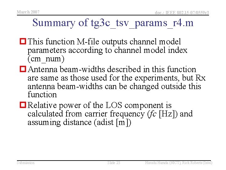
March 2007 doc. : IEEE 802. 15 -07/0559 r 3 Summary of tg 3 c_tsv_params_r 4. m p This function M-file outputs channel model parameters according to channel model index (cm_num) p Antenna beam-widths described in this function are same as those used for the experiments, but Rx antenna beam-widths can be changed outside this function p Relative power of the LOS component is calculated from carrier frequency (fc [Hz]) and assuming distance (adist [m]) Submission Slide 23 Hiroshi Harada (NICT), Rick Roberts (Intel)

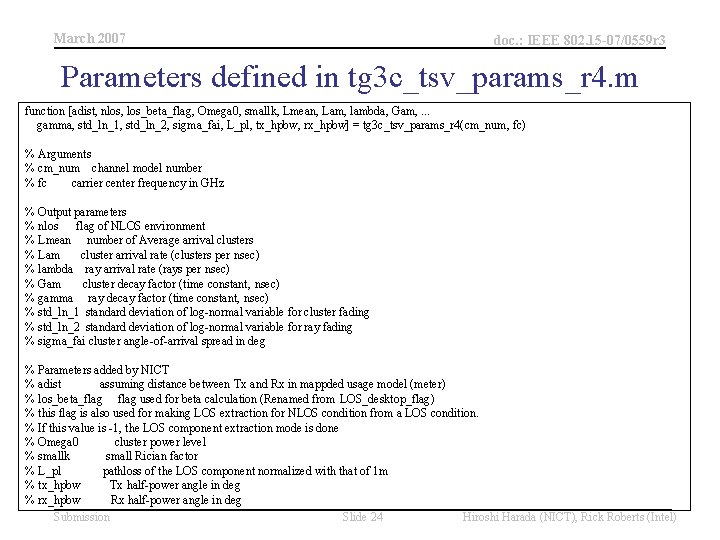
March 2007 doc. : IEEE 802. 15 -07/0559 r 3 Parameters defined in tg 3 c_tsv_params_r 4. m function [adist, nlos, los_beta_flag, Omega 0, smallk, Lmean, Lam, lambda, Gam, . . . gamma, std_ln_1, std_ln_2, sigma_fai, L_pl, tx_hpbw, rx_hpbw] = tg 3 c_tsv_params_r 4(cm_num, fc) % Arguments % cm_num channel model number % fc carrier center frequency in GHz % Output parameters % nlos flag of NLOS environment % Lmean number of Average arrival clusters % Lam cluster arrival rate (clusters per nsec) % lambda ray arrival rate (rays per nsec) % Gam cluster decay factor (time constant, nsec) % gamma ray decay factor (time constant, nsec) % std_ln_1 standard deviation of log-normal variable for cluster fading % std_ln_2 standard deviation of log-normal variable for ray fading % sigma_fai cluster angle-of-arrival spread in deg % Parameters added by NICT % adist assuming distance between Tx and Rx in mappded usage model (meter) % los_beta_flag used for beta calculation (Renamed from LOS_desktop_flag) % this flag is also used for making LOS extraction for NLOS condition from a LOS condition. % If this value is -1, the LOS component extraction mode is done % Omega 0 cluster power level % smallk small Rician factor % L_pl pathloss of the LOS component normalized with that of 1 m % tx_hpbw Tx half-power angle in deg % rx_hpbw Rx half-power angle in deg Submission Slide 24 Hiroshi Harada (NICT), Rick Roberts (Intel)

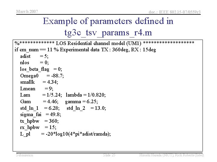
March 2007 doc. : IEEE 802. 15 -07/0559 r 3 Example of parameters defined in tg 3 c_tsv_params_r 4. m %******* LOS Residential channel model (UM 1) ********** if cm_num == 11 % Experimental data TX : 360 deg, RX : 15 deg adist = 5; nlos = 0; los_beta_flag = 0; Omega 0 = -88. 7; smallk = 4. 34; Lmean = 9; Lam = 1/5. 24; lambda = 1/0. 820; Gam = 4. 46; gamma = 6. 25; std_ln_1 = 6. 28; std_ln_2 = 13. 0; sigma_fai = 49. 8; tx_hpbw = 360; rx_hpbw = 15; L_pl = -20*log 10(4*pi*adist/ramda); Submission Slide 25 Hiroshi Harada (NICT), Rick Roberts (Intel)

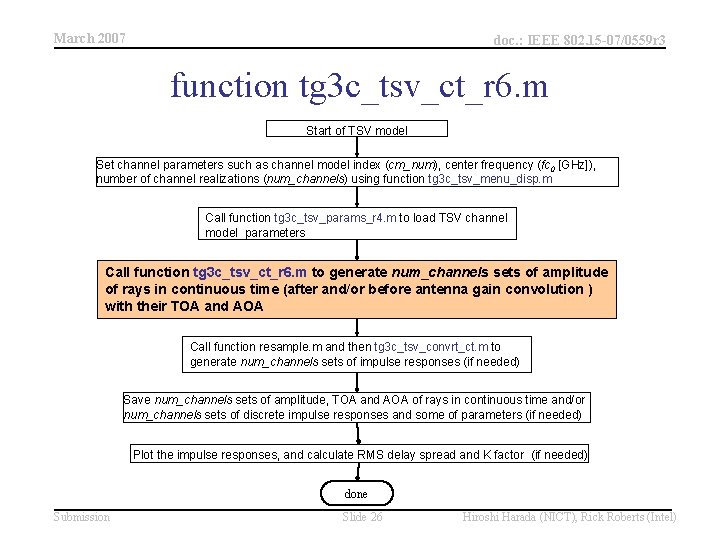
March 2007 doc. : IEEE 802. 15 -07/0559 r 3 function tg 3 c_tsv_ct_r 6. m Start of TSV model Set channel parameters such as channel model index (cm_num), center frequency (fc 0 [GHz]), number of channel realizations (num_channels) using function tg 3 c_tsv_menu_disp. m Call function tg 3 c_tsv_params_r 4. m to load TSV channel model parameters Call function tg 3 c_tsv_ct_r 6. m to generate num_channels sets of amplitude of rays in continuous time (after and/or before antenna gain convolution ) with their TOA and AOA Call function resample. m and then tg 3 c_tsv_convrt_ct. m to generate num_channels sets of impulse responses (if needed) Save num_channels sets of amplitude, TOA and AOA of rays in continuous time and/or num_channels sets of discrete impulse responses and some of parameters (if needed) Plot the impulse responses, and calculate RMS delay spread and K factor (if needed) done Submission Slide 26 Hiroshi Harada (NICT), Rick Roberts (Intel)

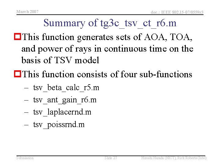
March 2007 doc. : IEEE 802. 15 -07/0559 r 3 Summary of tg 3 c_tsv_ct_r 6. m p. This function generates sets of AOA, TOA, and power of rays in continuous time on the basis of TSV model p. This function consists of four sub-functions – – tsv_beta_calc_r 5. m tsv_ant_gain_r 6. m tsv_laplacernd. m tsv_poissrnd. m Submission Slide 27 Hiroshi Harada (NICT), Rick Roberts (Intel)

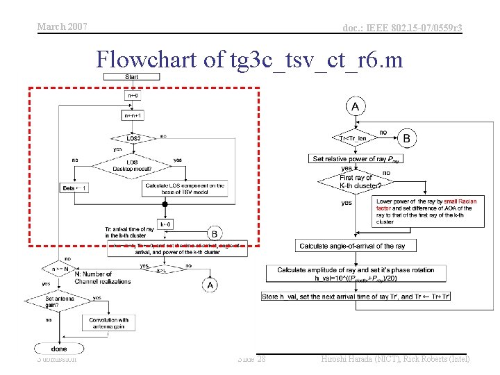
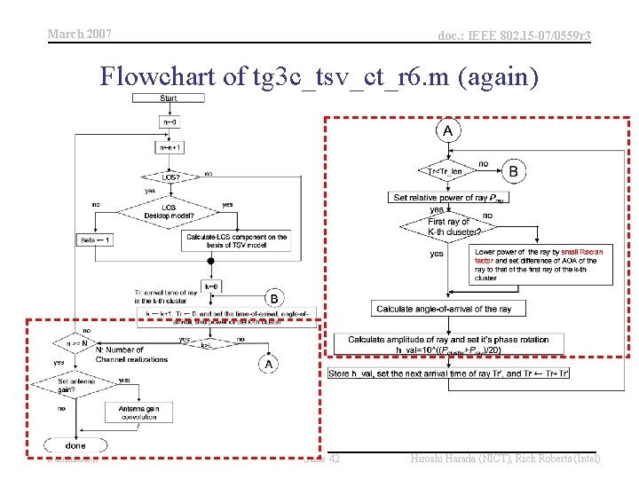
March 2007 doc. : IEEE 802. 15 -07/0559 r 3 Flowchart of tg 3 c_tsv_ct_r 6. m Submission Slide 28 Hiroshi Harada (NICT), Rick Roberts (Intel)

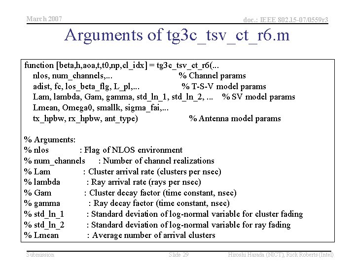
March 2007 doc. : IEEE 802. 15 -07/0559 r 3 Arguments of tg 3 c_tsv_ct_r 6. m function [beta, h, aoa, t, t 0, np, cl_idx] = tg 3 c_tsv_ct_r 6(. . . nlos, num_channels, . . . % Channel params adist, fc, los_beta_flg, L_pl, . . . % T-S-V model params Lam, lambda, Gam, gamma, std_ln_1, std_ln_2, . . . % SV model params Lmean, Omega 0, smallk, sigma_fai, . . . tx_hpbw, rx_hpbw, ant_type) % Antenna model params % Arguments: % nlos : Flag of NLOS environment % num_channels : Number of channel realizations % Lam : Cluster arrival rate (clusters per nsec) % lambda : Ray arrival rate (rays per nsec) % Gam : Cluster decay factor (time constant, nsec) % gamma : Ray decay factor (time constant, nsec) % std_ln_1 : Standard deviation of log-normal variable for cluster fading % std_ln_2 : Standard deviation of log-normal variable for ray fading % Lmean : Average number of arrival clusters Submission Slide 29 Hiroshi Harada (NICT), Rick Roberts (Intel)

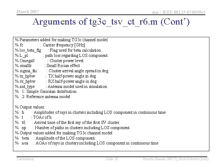
March 2007 doc. : IEEE 802. 15 -07/0559 r 3 Arguments of tg 3 c_tsv_ct_r 6. m (Cont’) % Parameters added for making TG 3 c channel model % fc : Carrier frequency [GHz] % los_beta_flg : Flag used for beta calculation % L_pl : path loss regarding LOS component % Omega 0 : Cluster power level % smallk : Small Rician effect % sigma_fai : Cluster arrival angle spread in deg % tx_hpbw : TX half-power angle in deg % rx_hpbw : RX half-power angle in deg % ant_type : Antenna model used in simulation % 1: Simple Gaussian distribution % 2: Reference antenna model % Output values: % h : Amplitudes of rays in clusters including LOS component in continuous time % t : TOAs of h % t 0 : Arrival time of the first ray of the first SV cluster % np : Number of paths in clusters including LOS component % Output values added for making TG 3 c channel model % beta : Amplitude of the LOS component % aoa : AOAs of rays in clusters including LOS component in continuous time Submission Slide 30 Hiroshi Harada (NICT), Rick Roberts (Intel)

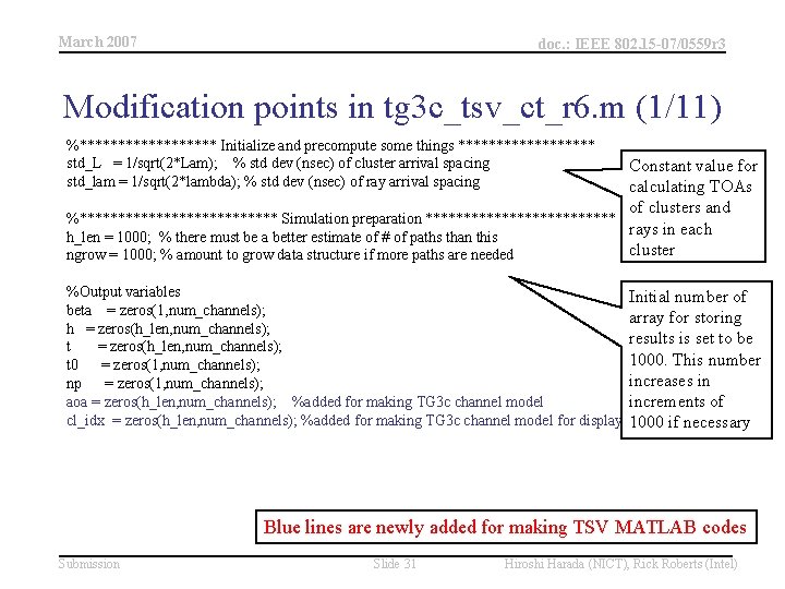
March 2007 doc. : IEEE 802. 15 -07/0559 r 3 Modification points in tg 3 c_tsv_ct_r 6. m (1/11) %********* Initialize and precompute some things ********* std_L = 1/sqrt(2*Lam); % std dev (nsec) of cluster arrival spacing std_lam = 1/sqrt(2*lambda); % std dev (nsec) of ray arrival spacing Constant value for calculating TOAs of clusters and %************* Simulation preparation ************* rays in each h_len = 1000; % there must be a better estimate of # of paths than this cluster ngrow = 1000; % amount to grow data structure if more paths are needed %Output variables beta = zeros(1, num_channels); h = zeros(h_len, num_channels); t 0 = zeros(1, num_channels); np = zeros(1, num_channels); aoa = zeros(h_len, num_channels); %added for making TG 3 c channel model cl_idx = zeros(h_len, num_channels); %added for making TG 3 c channel model for display Initial number of array for storing results is set to be 1000. This number increases in increments of 1000 if necessary Blue lines are newly added for making TSV MATLAB codes Submission Slide 31 Hiroshi Harada (NICT), Rick Roberts (Intel)

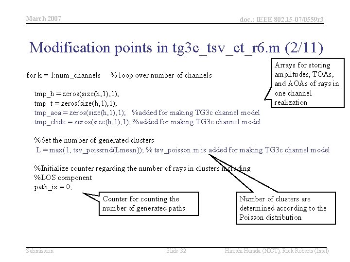
March 2007 doc. : IEEE 802. 15 -07/0559 r 3 Modification points in tg 3 c_tsv_ct_r 6. m (2/11) for k = 1: num_channels % loop over number of channels tmp_h = zeros(size(h, 1); tmp_t = zeros(size(h, 1); tmp_aoa = zeros(size(h, 1); %added for making TG 3 c channel model tmp_clidx = zeros(size(h, 1); %added for making TG 3 c channel model Arrays for storing amplitudes, TOAs, and AOAs of rays in one channel realization %Set the number of generated clusters L = max(1, tsv_poissrnd(Lmean)); % tsv_poisson. m is added for making TG 3 c channel model %Initialize counter regarding the number of rays in clusters including %LOS component path_ix = 0; Counter for counting the number of generated paths Submission Slide 32 Number of clusters are determined according to the Poisson distribution Hiroshi Harada (NICT), Rick Roberts (Intel)

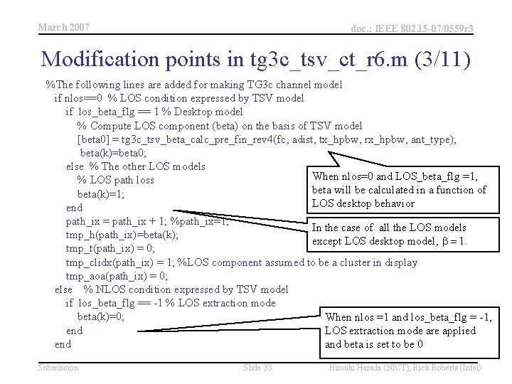
March 2007 doc. : IEEE 802. 15 -07/0559 r 3 Modification points in tg 3 c_tsv_ct_r 6. m (3/11) %The following lines are added for making TG 3 c channel model if nlos==0 % LOS condition expressed by TSV model if los_beta_flg == 1 % Desktop model % Compute LOS component (beta) on the basis of TSV model [beta 0] = tg 3 c_tsv_beta_calc_pre_fin_rev 4(fc, adist, tx_hpbw, rx_hpbw, ant_type); beta(k)=beta 0; else % The other LOS models When nlos=0 and LOS_beta_flg =1, % LOS path loss beta will be calculated in a function of beta(k)=1; LOS desktop behavior end path_ix = path_ix + 1; %path_ix=1; In the case of all the LOS models tmp_h(path_ix)=beta(k); except LOS desktop model, b = 1. tmp_t(path_ix) = 0; tmp_clidx(path_ix) = 1; %LOS component assumed to be a cluster in display tmp_aoa(path_ix) = 0; else % NLOS condition expressed by TSV model if los_beta_flg == -1 % LOS extraction mode beta(k)=0; When nlos =1 and los_beta_flg = -1, end LOS extraction mode are applied end and beta is set to be 0 Submission Slide 33 Hiroshi Harada (NICT), Rick Roberts (Intel)

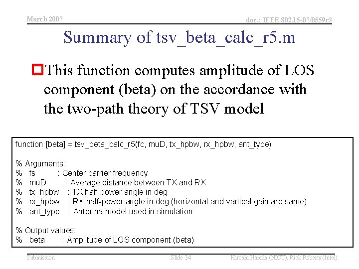
March 2007 doc. : IEEE 802. 15 -07/0559 r 3 Summary of tsv_beta_calc_r 5. m p. This function computes amplitude of LOS component (beta) on the accordance with the two-path theory of TSV model function [beta] = tsv_beta_calc_r 5(fc, mu. D, tx_hpbw, rx_hpbw, ant_type) % Arguments: % fs : Center carrier frequency % mu. D : Average distance between TX and RX % tx_hpbw : TX half-power angle in deg % rx_hpbw : RX half-power angle in deg (horizontal and vartical gain are same) % ant_type : Antenna model used in simulation % Output values: % beta : Amplitude of LOS component (beta) Submission Slide 34 Hiroshi Harada (NICT), Rick Roberts (Intel)

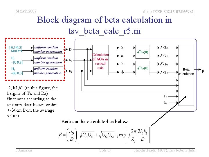
March 2007 doc. : IEEE 802. 15 -07/0559 r 3 Block diagram of beta calculation in tsv_beta_calc_r 5. m D, h 1, h 2 (in this figure, the heights of Tx and Rx) fluctuates according to the uniform distribution within +-30 cm from the average value) Beta can be calculated as below. Submission Slide 35 Hiroshi Harada (NICT), Rick Roberts (Intel)

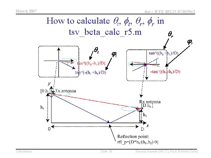
March 2007 doc. : IEEE 802. 15 -07/0559 r 3 How to calculate qt, ft, qr, fr in tsv_beta_calc_r 5. m qt qr jr jt D Submission Slide 36 Hiroshi Harada (NICT), Rick Roberts (Intel)

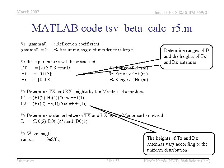
March 2007 doc. : IEEE 802. 15 -07/0559 r 3 MATLAB code tsv_beta_calc_r 5. m % gamma 0 : Reflection coefficient gamma 0 = 1; % Assuming angle of incidence is large % these parameters will be discussed D 0 = [-0. 3]+mu. D; Ht = [0 0. 3]; Hr = [0 0. 3]; % Range of D (m) % Range of Ht (m) % Range of Hr (m) Determine ranges of D and the heights of Tx and Rx antennas % Determine TX and RX heights by the Monte-carlo method h 1 = (Ht(2)-Ht(1))*rand+Ht(1); h 2 = (Hr(2)-Hr(1))*rand+Hr(1); % Determine distance between TX and RX by the Monte-carlo method D = (D 0(2)-D 0(1))*rand+D 0(1); % Wave length ramda = 3 e 8/fc; Submission The heights of Tx and Rx antennas vary according to the uniform distribution Slide 37 Hiroshi Harada (NICT), Rick Roberts (Intel)

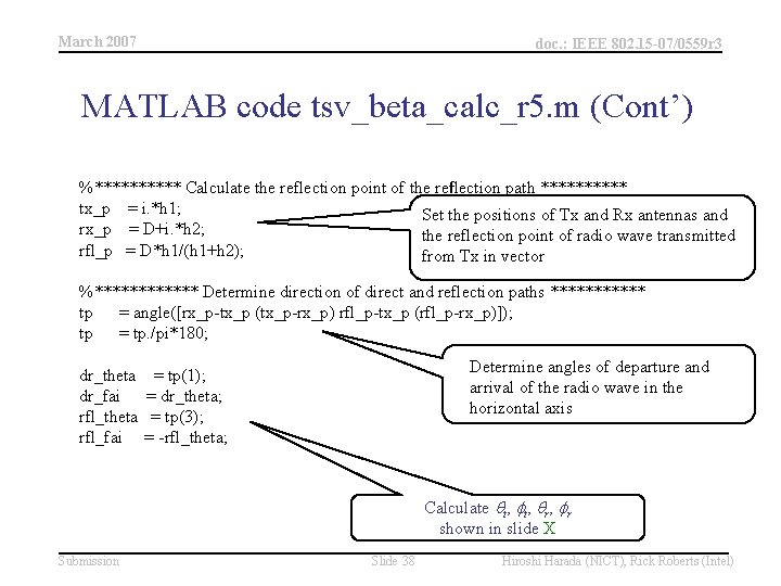
March 2007 doc. : IEEE 802. 15 -07/0559 r 3 MATLAB code tsv_beta_calc_r 5. m (Cont’) %***** Calculate the reflection point of the reｆlection path ***** tx_p = i. *h 1; Set the positions of Tx and Rx antennas and rx_p = D+i. *h 2; the reflection point of radio wave transmitted rfl_p = D*h 1/(h 1+h 2); from Tx in vector %****** Determine direction of direct and reflection paths ****** tp = angle([rx_p-tx_p (tx_p-rx_p) rfl_p-tx_p (rfl_p-rx_p)]); tp = tp. /pi*180; dr_theta dr_fai rfl_theta rfl_fai Determine angles of departure and arrival of the radio wave in the horizontal axis = tp(1); = dr_theta; = tp(3); = -rfl_theta; Calculate qt, ft, qr, fr shown in slide X Submission Slide 38 Hiroshi Harada (NICT), Rick Roberts (Intel)

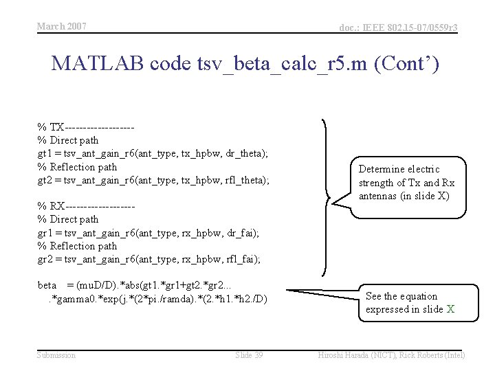
March 2007 doc. : IEEE 802. 15 -07/0559 r 3 MATLAB code tsv_beta_calc_r 5. m (Cont’) % TX---------% Direct path gt 1 = tsv_ant_gain_r 6(ant_type, tx_hpbw, dr_theta); % Reflection path gt 2 = tsv_ant_gain_r 6(ant_type, tx_hpbw, rfl_theta); % RX---------% Direct path gr 1 = tsv_ant_gain_r 6(ant_type, rx_hpbw, dr_fai); % Reflection path gr 2 = tsv_ant_gain_r 6(ant_type, rx_hpbw, rfl_fai); beta = (mu. D/D). *abs(gt 1. *gr 1+gt 2. *gr 2. . *gamma 0. *exp(j. *(2*pi. /ramda). *(2. *h 1. *h 2. /D) Submission Slide 39 Determine electric strength of Tx and Rx antennas (in slide X) See the equation expressed in slide X Hiroshi Harada (NICT), Rick Roberts (Intel)

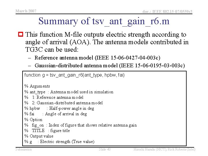
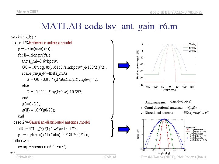
March 2007 doc. : IEEE 802. 15 -07/0559 r 3 Summary of tsv_ant_gain_r 6. m p This function M-file outputs electric strength according to angle of arrival (AOA). The antenna models contributed in TG 3 C can be used: – Reference antenna model (IEEE 15 -06 -0427 -04 -003 c) – Gaussian-distributed antenna model (IEEE 15 -06 -0195 -03 -003 c) function g = tsv_ant_gain_r 6(ant_type, hpbw, fai) % Arguments % ant_type : Antenna model used in simulation % 1: Reference antenna model % 2: Gaussian-distributed antenna model % hpbw : Half-power angle in deg % fai : Angle of arrival in deg % Option % fig_on : Index of figure that shows relative antenna gain % TITLE : figure title % Output value % g : Electric strength (True value) Submission Slide 40 Hiroshi Harada (NICT), Rick Roberts (Intel)

March 2007 doc. : IEEE 802. 15 -07/0559 r 3 MATLAB code tsv_ant_gain_r 6. m switch ant_type case 1 %Reference antenna model g = zeros(size(fai)); for ii=1: length(fai) theta_ml=2. 6*hpbw; G 0 = 10*log 10((1. 6162. /sin(hpbw*pi/180/2))^2); if abs(fai(ii))<=theta_ml/2 G = G 0 - 3. 01 * (2*abs(fai(ii)). /hpbw). ^2; else G = -0. 4111. *log(hpbw)-10. 597; end g 0=G-G 0; g(ii) = 10. ^(g 0/20); end case 2 %Gaussian-distributed antenna model alfa = 4*log(2). /(hpbw*pi/180). ^2; g = sqrt(exp(-alfa. *abs(fai. /180*pi). ^2)); otherwise error('Antenna model error') end Submission Slide 41 Hiroshi Harada (NICT), Rick Roberts (Intel)

March 2007 doc. : IEEE 802. 15 -07/0559 r 3 Flowchart of tg 3 c_tsv_ct_r 6. m (again) Submission Slide 42 Hiroshi Harada (NICT), Rick Roberts (Intel)

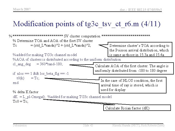
March 2007 doc. : IEEE 802. 15 -07/0559 r 3 Modification points of tg 3 c_tsv_ct_r 6. m (4/11) %************* SV cluster computation ************* % Determine TOA and AOA of the fisrt SV cluster Tc = (std_L*randn)^2 + (std_L*randn)^2; Determine cluster’s TOA according to the Poisson arrival distribution, which %added for making TG 3 c channel model is same as those in 15. 3 a and 15. 4 a %AOA of clusters is distributed according to the uniform distribution cl_ang_deg = 360*rand-180; Calculate AOA of the first cluster. The angle is uniformly distributed from -180 to 180 degree if nlos == 1 && los_beta_flg == -1 t 0(k) = Tc; end In the case of NLOS condition, the first arrival time of ray is stored, which is used for display % delta K factor d. K = L_pl-Omega 0; %added for making TG 3 c channel model Tc 0 = Tc; Calculate Rician factor (d. K) Submission Slide 43 Hiroshi Harada (NICT), Rick Roberts (Intel)

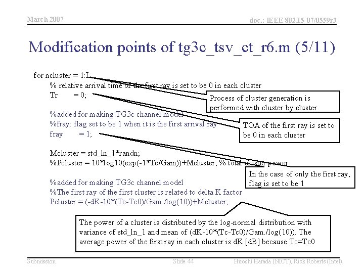
March 2007 doc. : IEEE 802. 15 -07/0559 r 3 Modification points of tg 3 c_tsv_ct_r 6. m (5/11) for ncluster = 1: L % relative arrival time of the first ray is set to be 0 in each cluster Tr = 0; Process of cluster generation is performed with cluster by cluster %added for making TG 3 c channel model %fray: flag set to be 1 when it is the first arrival ray TOA of the first ray is set to fray = 1; be 0 in each cluster Mcluster = std_ln_1*randn; %Pcluster = 10*log 10(exp(-1*Tc/Gam))+Mcluster; % total cluster power In the case of only the first ray, %added for making TG 3 c channel model flag is set to be 1 %The first ray of the first cluster is related to delta K factor Pcluster = (-d. K-10*(Tc-Tc 0)/Gam. /log(10))+Mcluster; The power of a cluster is distributed by the log-normal distribution with variance of std_ln_1 and mean of (d. K-10*(Tc-Tc 0)/Gam. /log(10)). The average power of the first ray in each cluster is d. K [d. B] because Tc=Tc 0 Submission Slide 44 Hiroshi Harada (NICT), Rick Roberts (Intel)

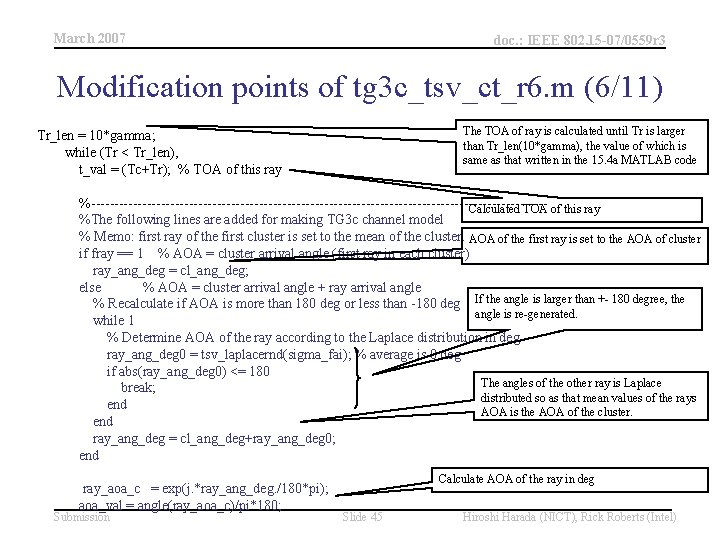
March 2007 doc. : IEEE 802. 15 -07/0559 r 3 Modification points of tg 3 c_tsv_ct_r 6. m (6/11) The TOA of ray is calculated until Tr is larger than Tr_len(10*gamma), the value of which is same as that written in the 15. 4 a MATLAB code Tr_len = 10*gamma; while (Tr < Tr_len), t_val = (Tc+Tr); % TOA of this ray %-------------------------------------------------Calculated TOA of this ray %The following lines are added for making TG 3 c channel model % Memo: first ray of the first cluster is set to the mean of the cluster. AOA of the first ray is set to the AOA of cluster if fray == 1 % AOA = cluster arrival angle (first ray in each cluster) ray_ang_deg = cl_ang_deg; else % AOA = cluster arrival angle + ray arrival angle % Recalculate if AOA is more than 180 deg or less than -180 deg If the angle is larger than +- 180 degree, the angle is re-generated. while 1 % Determine AOA of the ray according to the Laplace distribution in deg ray_ang_deg 0 = tsv_laplacernd(sigma_fai); % average is 0 deg if abs(ray_ang_deg 0) <= 180 The angles of the other ray is Laplace break; distributed so as that mean values of the rays end AOA is the AOA of the cluster. end ray_ang_deg = cl_ang_deg+ray_ang_deg 0; end ray_aoa_c = exp(j. *ray_ang_deg. /180*pi); aoa_val = angle(ray_aoa_c)/pi*180; Submission Calculate AOA of the ray in deg Slide 45 Hiroshi Harada (NICT), Rick Roberts (Intel)

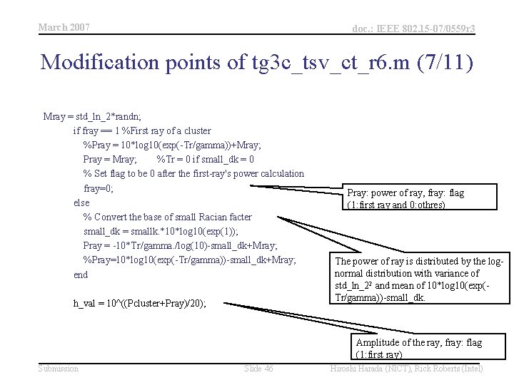
March 2007 doc. : IEEE 802. 15 -07/0559 r 3 Modification points of tg 3 c_tsv_ct_r 6. m (7/11) Mray = std_ln_2*randn; if fray == 1 %First ray of a cluster %Pray = 10*log 10(exp(-Tr/gamma))+Mray; Pray = Mray; %Tr = 0 if small_dk = 0 % Set flag to be 0 after the first-ray's power calculation fray=0; else % Convert the base of small Racian facter small_dk = smallk. *10*log 10(exp(1)); Pray = -10*Tr/gamma. /log(10)-small_dk+Mray; %Pray=10*log 10(exp(-Tr/gamma))-small_dk+Mray; end h_val = 10^((Pcluster+Pray)/20); Pray: power of ray, fray: flag (1: first ray and 0: othres) The power of ray is distributed by the lognormal distribution with variance of std_ln_22 and mean of 10*log 10(exp(Tr/gamma))-small_dk. Amplitude of the ray, fray: flag (1: first ray) Submission Slide 46 Hiroshi Harada (NICT), Rick Roberts (Intel)

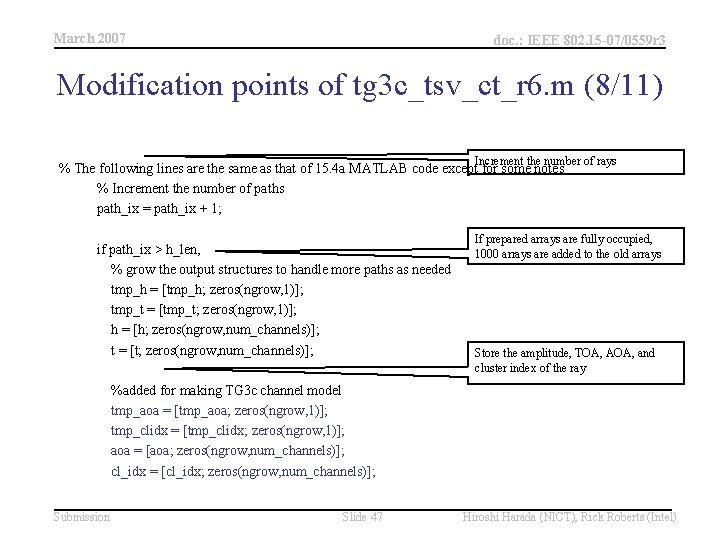
March 2007 doc. : IEEE 802. 15 -07/0559 r 3 Modification points of tg 3 c_tsv_ct_r 6. m (8/11) Increment the number of rays % The following lines are the same as that of 15. 4 a MATLAB code except for some notes % Increment the number of paths path_ix = path_ix + 1; if path_ix > h_len, % grow the output structures to handle more paths as needed tmp_h = [tmp_h; zeros(ngrow, 1)]; tmp_t = [tmp_t; zeros(ngrow, 1)]; h = [h; zeros(ngrow, num_channels)]; t = [t; zeros(ngrow, num_channels)]; If prepared arrays are fully occupied, 1000 arrays are added to the old arrays Store the amplitude, TOA, AOA, and cluster index of the ray %added for making TG 3 c channel model tmp_aoa = [tmp_aoa; zeros(ngrow, 1)]; tmp_clidx = [tmp_clidx; zeros(ngrow, 1)]; aoa = [aoa; zeros(ngrow, num_channels)]; cl_idx = [cl_idx; zeros(ngrow, num_channels)]; Submission Slide 47 Hiroshi Harada (NICT), Rick Roberts (Intel)

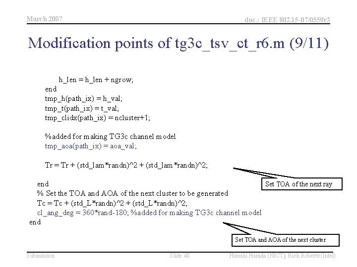
March 2007 doc. : IEEE 802. 15 -07/0559 r 3 Modification points of tg 3 c_tsv_ct_r 6. m (9/11) h_len = h_len + ngrow; end tmp_h(path_ix) = h_val; tmp_t(path_ix) = t_val; tmp_clidx(path_ix) = ncluster+1; %added for making TG 3 c channel model tmp_aoa(path_ix) = aoa_val; Tr = Tr + (std_lam*randn)^2; Set TOA of the next ray end % Set the TOA and AOA of the next cluster to be generated Tc = Tc + (std_L*randn)^2; cl_ang_deg = 360*rand-180; %added for making TG 3 c channel model end Set TOA and AOA of the next cluster Submission Slide 48 Hiroshi Harada (NICT), Rick Roberts (Intel)

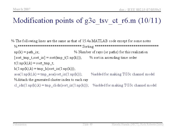
March 2007 doc. : IEEE 802. 15 -07/0559 r 3 Modification points of g 3 c_tsv_ct_r 6. m (10/11) % The following lines are the same as that of 15. 4 a MATLAB code except for some notes %***************** Sorting ***************** np(k) = path_ix; % Number of rays (or paths) for this realization [sort_tmp_t, sort_ix] = sort(tmp_t(1: np(k))); % sort in ascending time order t(1: np(k), k) = sort_tmp_t; h(1: np(k), k) = tmp_h(sort_ix(1: np(k))); aoa(1: np(k), k) = tmp_aoa(sort_ix(1: np(k))); %added for making TG 3 c channel model %Attach the generated cluster index to each ray cl_idx(1: np(k), k) = tmp_clidx(sort_ix(1: np(k))); %added for making TG 3 c channel model Submission Slide 49 Hiroshi Harada (NICT), Rick Roberts (Intel)

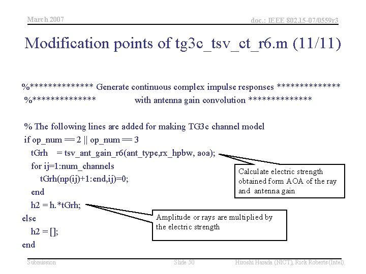
March 2007 doc. : IEEE 802. 15 -07/0559 r 3 Modification points of tg 3 c_tsv_ct_r 6. m (11/11) %******* Generate continuous complex impulse responses ******* %******* with antenna gain convolution ******* % The following lines are added for making TG 3 c channel model if op_num == 2 || op_num == 3 t. Grh = tsv_ant_gain_r 6(ant_type, rx_hpbw, aoa); for ij=1: num_channels Calculate electric strength t. Grh(np(ij)+1: end, ij)=0; obtained form AOA of the ray and antenna gain end h 2 = h. *t. Grh; Amplitude or rays are multiplied by else the electric strength h 2 = []; end Submission Slide 50 Hiroshi Harada (NICT), Rick Roberts (Intel)

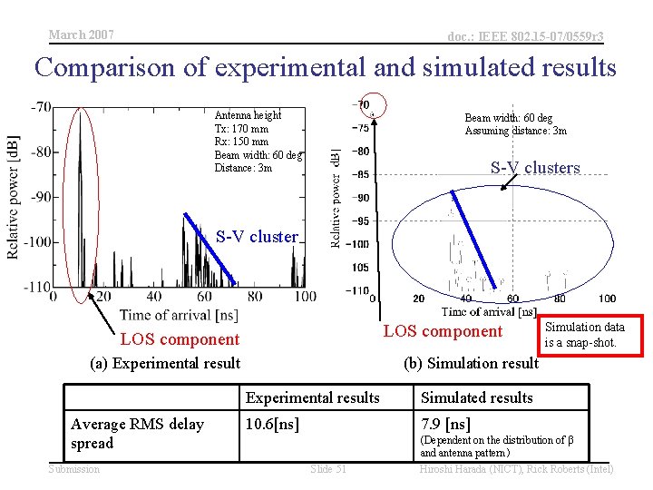
March 2007 doc. : IEEE 802. 15 -07/0559 r 3 Comparison of experimental and simulated results Antenna height Tx: 170 mm Rx: 150 mm Beam width: 60 deg Distance: 3 m Beam width: 60 deg Assuming distance: 3 m S-V clusters S-V cluster LOS component (a) Experimental result Average RMS delay spread Submission Simulation data is a snap-shot. (b) Simulation result Experimental results Simulated results 10. 6[ns] 7. 9 [ns] (Dependent on the distribution of β and antenna pattern） Slide 51 Hiroshi Harada (NICT), Rick Roberts (Intel)

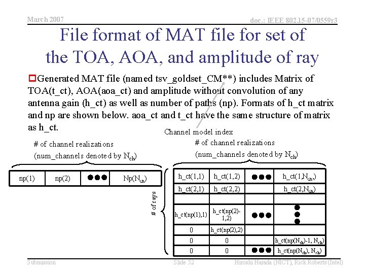
March 2007 doc. : IEEE 802. 15 -07/0559 r 3 File format of MAT file for set of the TOA, AOA, and amplitude of ray p. Generated MAT file (named tsv_goldset_CM**) includes Matrix of TOA(t_ct), AOA(aoa_ct) and amplitude without convolution of any antenna gain (h_ct) as well as number of paths (np). Formats of h_ct matrix and np are shown below. aoa_ct and t_ct have the same structure of matrix as h_ct. Channel model index # of channel realizations (num_channels denoted by Nch) np(2) Np(Nch) # of rays np(1) h_ct(1, 2) h_ct(1, Nch, ) h_ct(2, 1) h_ct(2, 2) h_ct(2, Nch) h_ct(np(1), 1) h_ct(np(2)1, 2) 0 0 0 Submission Slide 52 h_ct(np(2), 2) 0 0 h_ct(np(Nch)-1, Nch) h_ct(np(Nch), Nch) Hiroshi Harada (NICT), Rick Roberts (Intel)

March 2007 doc. : IEEE 802. 15 -07/0559 r 3 File format of MAT file for discrete impulse responses p. Generated MAT file (named tsv_d. IR_cm**_n*_at*_fs*) includes Discrete impulse responses (combined with convolution of antenna gain) (h). Format of h matrix is shown below. aoa_ct and t_ct have the same structure of matrix as h. Channel model index # of taps (dependent sample rate) # of channel realizations (num_channels denoted by Nch) Submission Number of channel realizations Antenna model Sample rate h(1, 1) h(1, 2) h(1, Nch, ) h(2, 1) h (2, 2) h(2, Nch) h(ngrow, 1) h(ngrow, 2) Slide 53 h(ngrow, Nch) Hiroshi Harada (NICT), Rick Roberts (Intel)

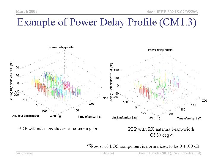
March 2007 doc. : IEEE 802. 15 -07/0559 r 3 Example of Power Delay Profile (CM 1. 3) PDP without convolution of antenna gain PDP with RX antenna beam-width Of 30 deg (*)Power Submission of LOS component is normalized to be 0 +100 d. B Slide 54 Hiroshi Harada (NICT), Rick Roberts (Intel)

March 2007 doc. : IEEE 802. 15 -07/0559 r 3 Summary of TSV channel model Matlab code p Explained the following items – – Overview , equations and parameters of TSV model Available channel models by TSV model Flowchart of the TSV model MATLAB code Primal functions in the program p Exhibited the following items – Comparison of experimental and simulated results – File format of saved MAT files – Power delay profile Submission Slide 55 Hiroshi Harada (NICT), Rick Roberts (Intel)

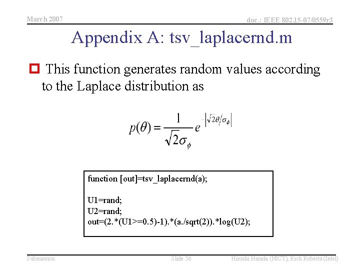
March 2007 doc. : IEEE 802. 15 -07/0559 r 3 Appendix A: tsv_laplacernd. m p This function generates random values according to the Laplace distribution as function [out]=tsv_laplacernd(a); U 1=rand; U 2=rand; out=(2. *(U 1>=0. 5)-1). *(a. /sqrt(2)). *log(U 2); Submission Slide 56 Hiroshi Harada (NICT), Rick Roberts (Intel)

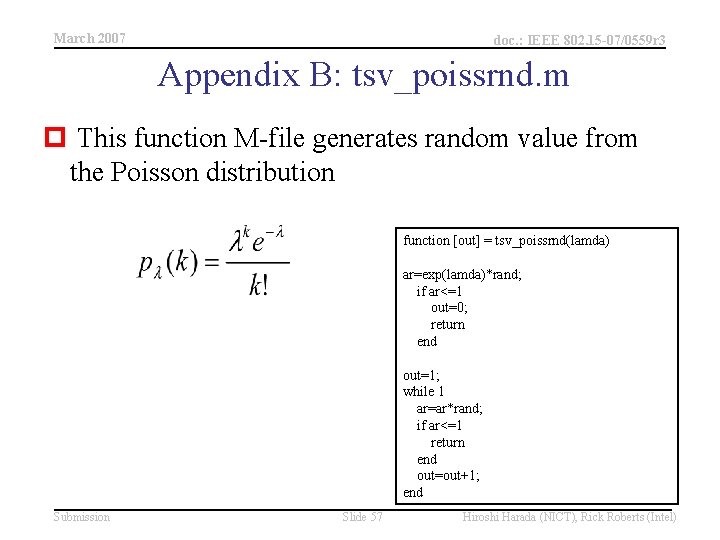
March 2007 doc. : IEEE 802. 15 -07/0559 r 3 Appendix B: tsv_poissrnd. m p This function M-file generates random value from the Poisson distribution function [out] = tsv_poissrnd(lamda) ar=exp(lamda)*rand; if ar<=1 out=0; return end out=1; while 1 ar=ar*rand; if ar<=1 return end out=out+1; end Submission Slide 57 Hiroshi Harada (NICT), Rick Roberts (Intel)

March 2007 doc. : IEEE 802. 15 -07/0559 r 3 Appendix C: tg 3 c_sv_cnvrt_ct. m p The function converts continuous-time channel model h_ct to N-times over-sampled discrete-time samples convert continuous-time channel model h_ct to N-times oversampled discrete-time samples h_ct, t, np, and num_channels are as specified in uwb_sv_model ts is the desired time resolution h. N will be produced with time resolution ts / N. p It is up to the user to then apply any filtering and/or complex down-conversion and then decimate by N to finally obtain an impulse response at time resolution ts. Submission Slide 58 Hiroshi Harada (NICT), Rick Roberts (Intel)

March 2007 doc. : IEEE 802. 15 -07/0559 r 3 Appendix D: tg 3 c_tsv_menu_disp. m and tg 3 c_tsv_results_disp. m p Tg 3 c_tsv_menu_disp. m, and tg 3 c_tsv_results_disp setups input arguments, and exhibits some of highlight simulation results, respectively Submission Slide 59 Hiroshi Harada (NICT), Rick Roberts (Intel)

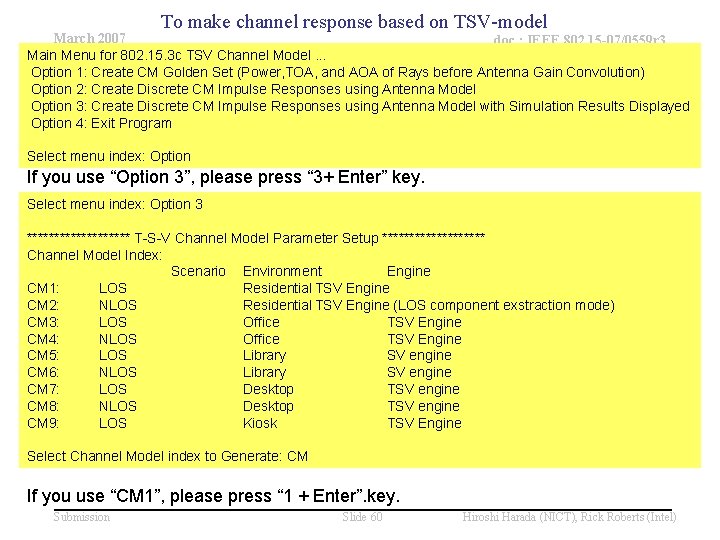
To make channel response based on TSV-model March 2007 doc. : IEEE 802. 15 -07/0559 r 3 Main Menu for 802. 15. 3 c TSV Channel Model. . . Option 1: Create CM Golden Set (Power, TOA, and AOA of Rays before Antenna Gain Convolution) Option 2: Create Discrete CM Impulse Responses using Antenna Model Option 3: Create Discrete CM Impulse Responses using Antenna Model with Simulation Results Displayed Option 4: Exit Program Select menu index: Option If you use “Option 3”, please press “ 3+ Enter” key. Select menu index: Option 3 ********** T-S-V Channel Model Parameter Setup ********** Channel Model Index: Scenario Environment Engine CM 1: LOS Residential TSV Engine CM 2: NLOS Residential TSV Engine (LOS component exstraction mode) CM 3: LOS Office TSV Engine CM 4: NLOS Office TSV Engine CM 5: LOS Library SV engine CM 6: NLOS Library SV engine CM 7: LOS Desktop TSV engine CM 8: NLOS Desktop TSV engine CM 9: LOS Kiosk TSV Engine Select Channel Model index to Generate: CM If you use “CM 1”, please press “ 1 + Enter”. key. Submission Slide 60 Hiroshi Harada (NICT), Rick Roberts (Intel)

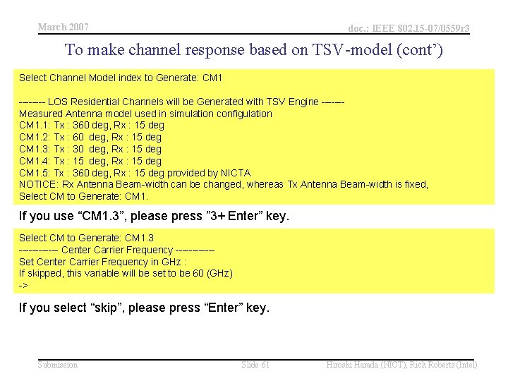
March 2007 doc. : IEEE 802. 15 -07/0559 r 3 To make channel response based on TSV-model (cont’) Select Channel Model index to Generate: CM 1 ---- LOS Residential Channels will be Generated with TSV Engine ------Measured Antenna model used in simulation configulation CM 1. 1: Tx : 360 deg, Rx : 15 deg CM 1. 2: Tx : 60 deg, Rx : 15 deg CM 1. 3: Tx : 30 deg, Rx : 15 deg CM 1. 4: Tx : 15 deg, Rx : 15 deg CM 1. 5: Tx : 360 deg, Rx : 15 deg provided by NICTA NOTICE: Rx Antenna Beam-width can be changed, whereas Tx Antenna Beam-width is fixed, Select CM to Generate: CM 1. If you use “CM 1. 3”, please press ” 3+ Enter” key. Select CM to Generate: CM 1. 3 ------ Center Carrier Frequency ------Set Center Carrier Frequency in GHz : If skipped, this variable will be set to be 60 (GHz) -> If you select “skip”, please press “Enter” key. Submission Slide 61 Hiroshi Harada (NICT), Rick Roberts (Intel)

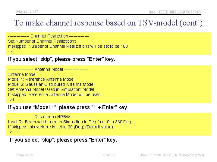
March 2007 doc. : IEEE 802. 15 -07/0559 r 3 To make channel response based on TSV-model (cont’) -------- Channel Realization -------Set Number of Channel Realizations If skipped, Number of Channel Realizations will be set to be 100 -> If you select “skip”, please press “Enter” key. --------- Antenna Model --------Antenna Model: Model 1: Reference Antenna Model 2: Gaussian-Distributed Antenna Model Set Antenna Model Used in Simulation: Model If skipped, Reference Antenna Model will be used ->1 If you use “Model 1”, please press ” 1 + Enter” key. --------- Rx antenna HPBW --------Input Rx Beam-width used in Simulation in Deg from 0 to 360 Deg If skipped, this variable is set to 30 (Deg) (Default value) -> If you select “skip”, please press “Enter” key. Submission Slide 62 Hiroshi Harada (NICT), Rick Roberts (Intel)

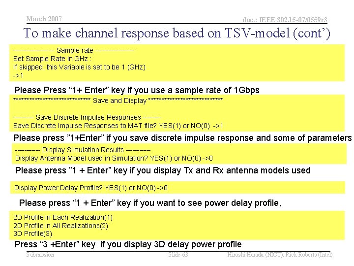
March 2007 doc. : IEEE 802. 15 -07/0559 r 3 To make channel response based on TSV-model (cont’) --------- Sample rate --------Set Sample Rate in GHz : If skipped, this Variable is set to be 1 (GHz) ->1 Please Press “ 1+ Enter” key if you use a sample rate of 1 Gbps *************** Save and Display ************** ----- Save Discrete Impulse Responses -------Save Discrete Impulse Responses to MAT file? YES(1) or NO(0) ->1 Please press ” 1+Enter” if you save discrete impulse response and some of parameters ------ Display Simulation Results -----Display Antenna Model used in Simulation? YES(1) or NO(0) ->0 Please press ” 1 + Enter” key if you display Tx and Rx antenna models used Display Power Delay Profile? YES(1) or NO(0) ->0 Please press “ 1 + Enter” key if you want to see power delay profile, 2 D Profile in Each Realization(1) 2 D Profile in All Realizations(2) 3 D Profile(3) Press “ 3 +Enter” key if you display 3 D delay power profile Submission Slide 63 Hiroshi Harada (NICT), Rick Roberts (Intel)

March 2007 doc. : IEEE 802. 15 -07/0559 r 3 SV Code Support Submission Slide 64 Hiroshi Harada (NICT), Rick Roberts (Intel)

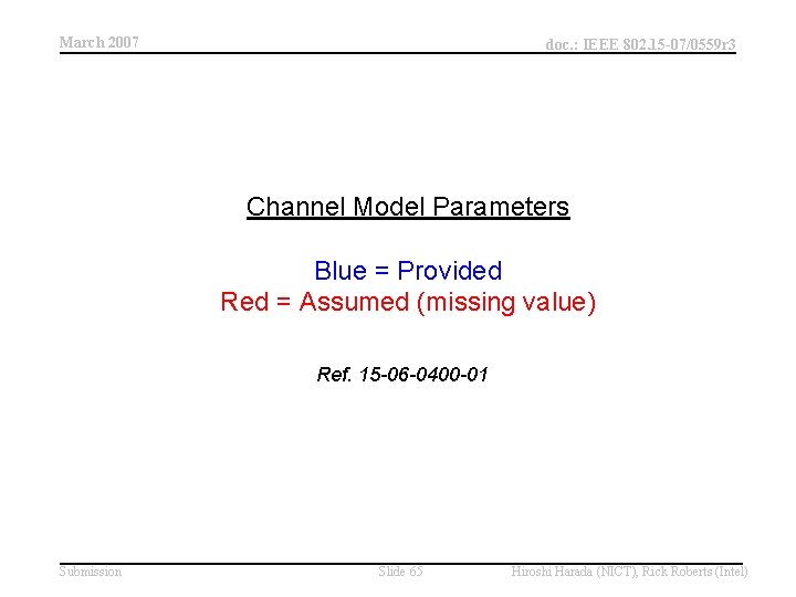
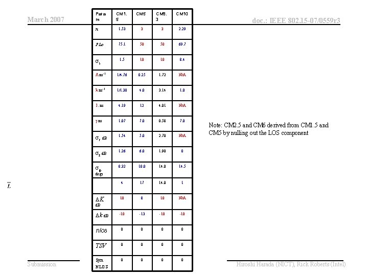
March 2007 doc. : IEEE 802. 15 -07/0559 r 3 Channel Model Parameters Blue = Provided Red = Assumed (missing value) Ref. 15 -06 -0400 -01 Submission Slide 65 Hiroshi Harada (NICT), Rick Roberts (Intel)

March 2007 Para m CM 1. 5 CM 9. 3 CM 10 doc. : IEEE 802. 15 -07/0559 r 3 n 1. 53 3 3 2. 29 PLo 75. 1 50 50 69. 7 s 1. 5 10 10 8. 4 L ns-1 1/4. 76 0. 25 1. 72 N/A l ns-1 1/1. 30 4. 0 3. 14 1. 0 1. ns 4. 19 12 4. 01 N/A g ns 1. 07 7. 0 0. 58 7. 0 c d. B 1. 54 5. 0 2. 70 N/A r d. B 1. 26 6. 0 1. 90 0 8. 32 10. 0 14. 5 4 17 14. 0 1 10 8 10 N/A k d. B -10 -13 -10 nlos 0 0 TSV 0 0 Syn NLOS 0 0 0 Note: CM 2. 5 and CM 6 derived from CM 1. 5 and CM 5 by nulling out the LOS component degs K d. B Submission 0 Slide 66 Hiroshi Harada (NICT), Rick Roberts (Intel)

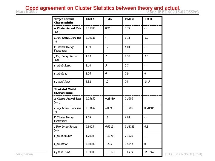
Good agreement on Cluster Statistics between theory and actual. March 2007 doc. : IEEE 802. 15 -07/0559 r 3 Target Channel Characteristics CM 1. 5 CM 9. 3 CM 10 Λ Cluster Arrival Rate (ns-1) 0. 21008 0. 25 1. 72 --- λ Ray Arrival Rate (ns -1) 0. 76923 4 3. 14 1. 0 Γ Cluster Decay Factor (ns) 4. 19 12 4. 01 --- γ Ray decay Factor (ns) 1. 07 7 0. 58 7. 0 σc sd of cluster 1. 54 5 2. 7 --- σr sd of ray 1. 26 6 1. 9 0 σΦ sd of Ao. A 8. 32 10 14 14. 5 Λ Cluster Arrival Rate (ns-1) 0. 15657 0. 23839 1. 5506 --- λ Ray Arrival Rate (ns -1) 0. 77449 4. 0098 3. 1296 0. 98505 Γ Cluster Decay Factor (ns) 4. 19 12 4. 01 --- γ Ray decay Factor (ns) 0. 8025 6. 6111 0. 54133 6. 8 σc sd of cluster 1. 2618 4. 1071 2. 1727 --- σr sd of ray 0. 98987 4. 785 1. 5243 0 σΦ sd of Ao. A 8. 3288 10. 0174 13. 977 Simulated Model Characteristics Submission Slide 67 14. 4369 Hiroshi Harada (NICT), Rick Roberts (Intel)

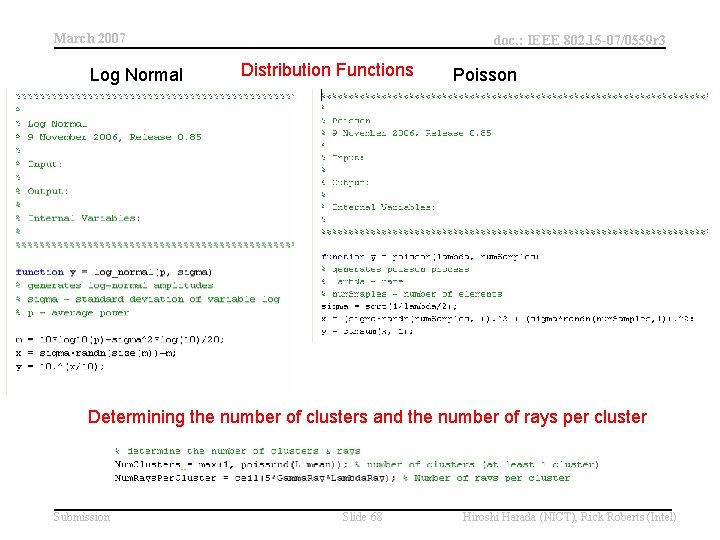
March 2007 Log Normal doc. : IEEE 802. 15 -07/0559 r 3 Distribution Functions Poisson Determining the number of clusters and the number of rays per cluster Submission Slide 68 Hiroshi Harada (NICT), Rick Roberts (Intel)

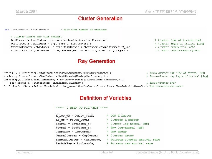
March 2007 doc. : IEEE 802. 15 -07/0559 r 3 Cluster Generation Ray Generation Definition of Variables Submission Slide 69 Hiroshi Harada (NICT), Rick Roberts (Intel)

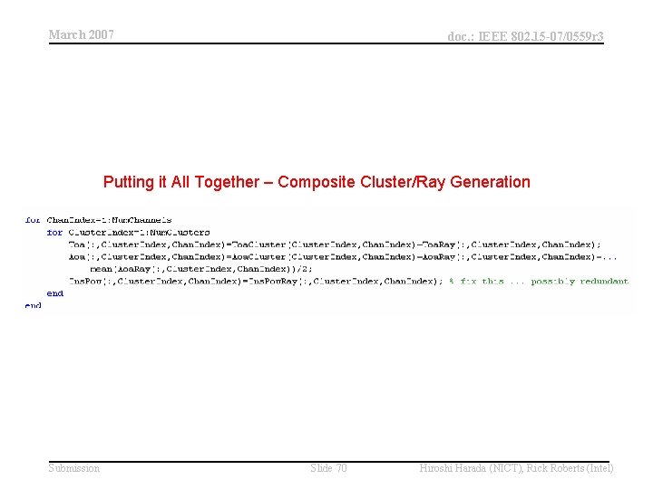
March 2007 doc. : IEEE 802. 15 -07/0559 r 3 Putting it All Together – Composite Cluster/Ray Generation Submission Slide 70 Hiroshi Harada (NICT), Rick Roberts (Intel)

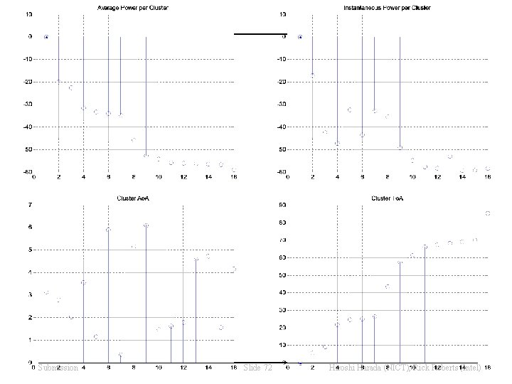
March 2007 doc. : IEEE 802. 15 -07/0559 r 3 Cluster Definition Submission Slide 71 Hiroshi Harada (NICT), Rick Roberts (Intel)

March 2007 Submission doc. : IEEE 802. 15 -07/0559 r 3 Slide 72 Hiroshi Harada (NICT), Rick Roberts (Intel)

March 2007 doc. : IEEE 802. 15 -07/0559 r 3 Ray Definition Submission Slide 73 Hiroshi Harada (NICT), Rick Roberts (Intel)

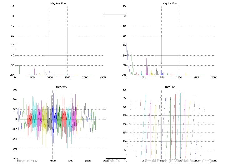
March 2007 Submission doc. : IEEE 802. 15 -07/0559 r 3 Slide 74 Hiroshi Harada (NICT), Rick Roberts (Intel)

March 2007 doc. : IEEE 802. 15 -07/0559 r 3 Combined Cluster + Ray Definition Submission Slide 75 Hiroshi Harada (NICT), Rick Roberts (Intel)

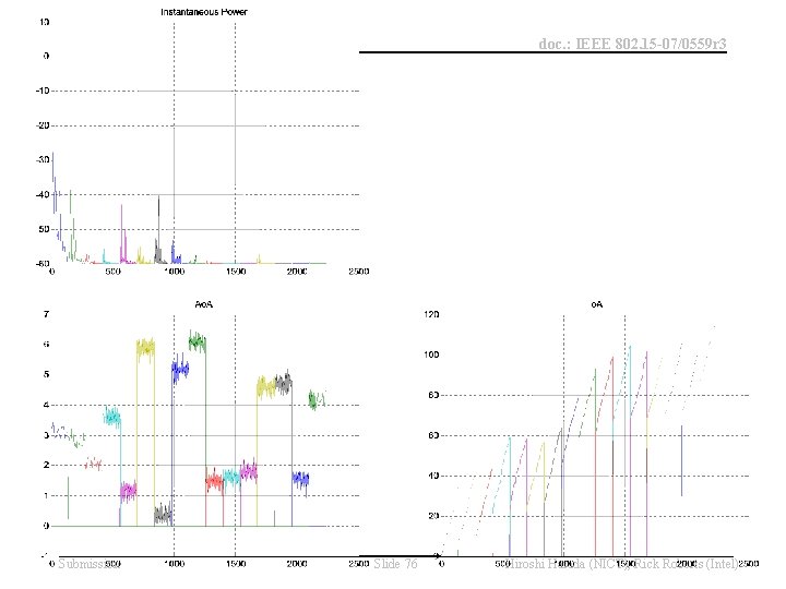
March 2007 Submission doc. : IEEE 802. 15 -07/0559 r 3 Slide 76 Hiroshi Harada (NICT), Rick Roberts (Intel)

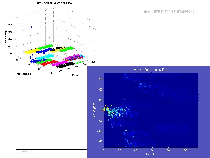
March 2007 doc. : IEEE 802. 15 -07/0559 r 3 3 -D Representation Submission Slide 77 Hiroshi Harada (NICT), Rick Roberts (Intel)

March 2007 Submission doc. : IEEE 802. 15 -07/0559 r 3 Slide 78 Hiroshi Harada (NICT), Rick Roberts (Intel)

March 2007 doc. : IEEE 802. 15 -07/0559 r 3 Discrete Time Sorted Definition Submission Slide 79 Hiroshi Harada (NICT), Rick Roberts (Intel)

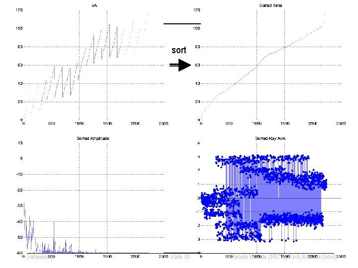
March 2007 doc. : IEEE 802. 15 -07/0559 r 3 sort Submission Slide 80 Hiroshi Harada (NICT), Rick Roberts (Intel)

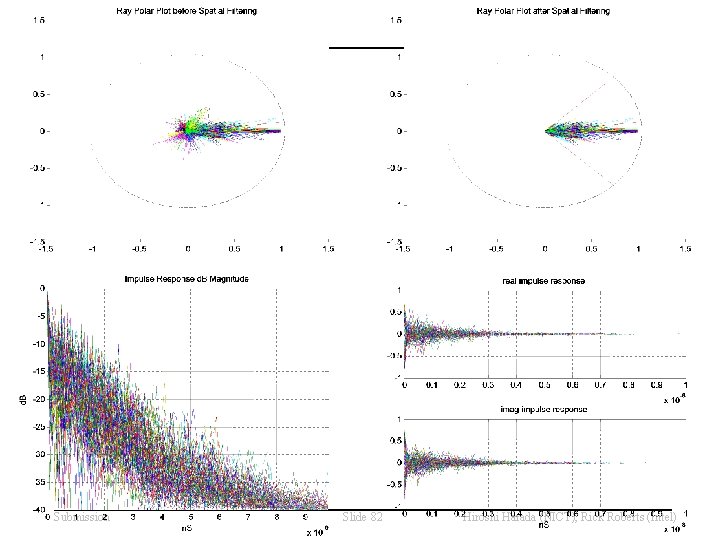
March 2007 doc. : IEEE 802. 15 -07/0559 r 3 Apply the Spatial Filtering to form IR Submission Slide 81 Hiroshi Harada (NICT), Rick Roberts (Intel)

March 2007 Submission doc. : IEEE 802. 15 -07/0559 r 3 Slide 82 Hiroshi Harada (NICT), Rick Roberts (Intel)

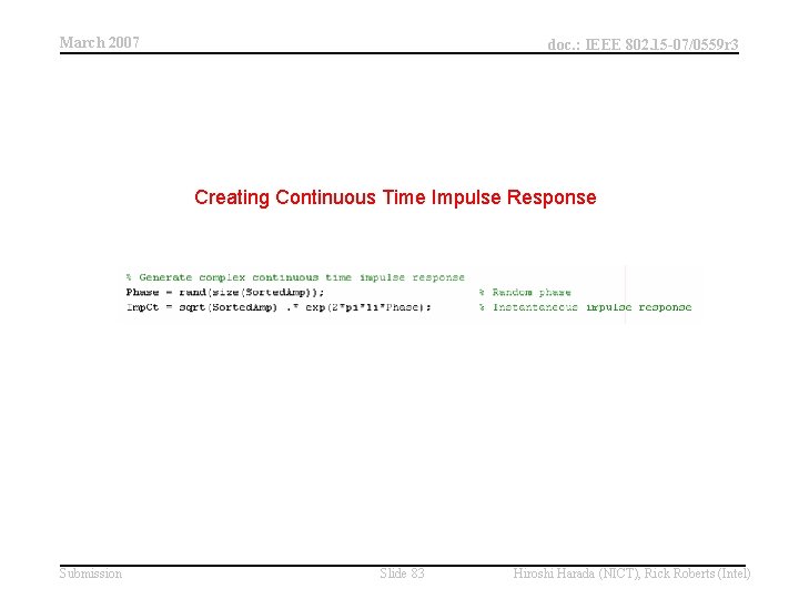
March 2007 doc. : IEEE 802. 15 -07/0559 r 3 Creating Continuous Time Impulse Response Submission Slide 83 Hiroshi Harada (NICT), Rick Roberts (Intel)

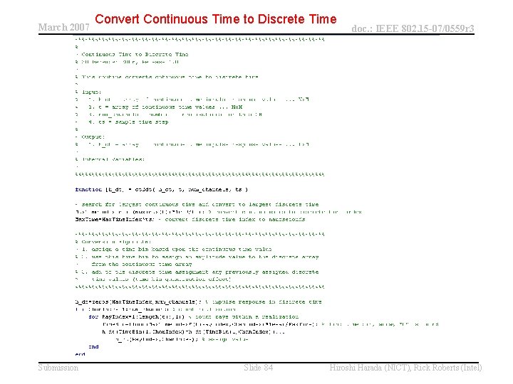
March 2007 Submission Convert Continuous Time to Discrete Time Slide 84 doc. : IEEE 802. 15 -07/0559 r 3 Hiroshi Harada (NICT), Rick Roberts (Intel)

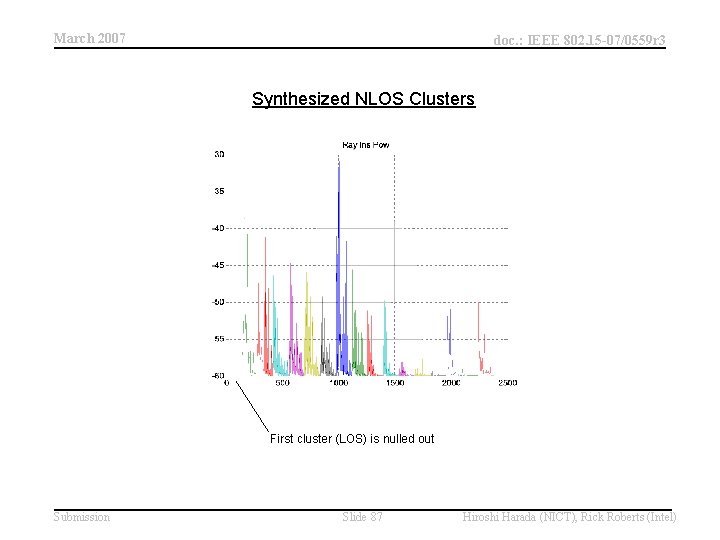
March 2007 doc. : IEEE 802. 15 -07/0559 r 3 Synthesizing NLOS Clusters from LOS Clusters Submission Slide 85 Hiroshi Harada (NICT), Rick Roberts (Intel)

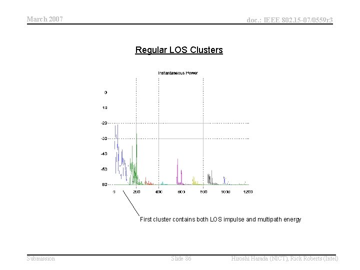
March 2007 doc. : IEEE 802. 15 -07/0559 r 3 Regular LOS Clusters First cluster contains both LOS impulse and multipath energy Submission Slide 86 Hiroshi Harada (NICT), Rick Roberts (Intel)

March 2007 doc. : IEEE 802. 15 -07/0559 r 3 Synthesized NLOS Clusters First cluster (LOS) is nulled out Submission Slide 87 Hiroshi Harada (NICT), Rick Roberts (Intel)

March 2007 doc. : IEEE 802. 15 -07/0559 r 3 Impulse Response Truncation Submission Slide 88 Hiroshi Harada (NICT), Rick Roberts (Intel)

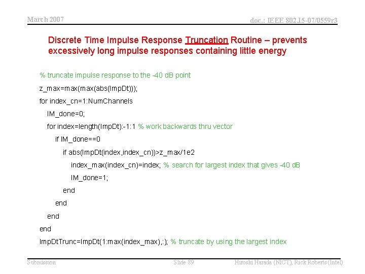
March 2007 doc. : IEEE 802. 15 -07/0559 r 3 Discrete Time Impulse Response Truncation Routine – prevents excessively long impulse responses containing little energy % truncate impulse response to the -40 d. B point z_max=max(abs(Imp. Dt))); for index_cn=1: Num. Channels IM_done=0; for index=length(Imp. Dt): -1: 1 % work backwards thru vector if IM_done==0 if abs(Imp. Dt(index, index_cn))>z_max/1 e 2 index_max(index_cn)=index; % search for largest index that gives -40 d. B IM_done=1; end end Imp. Dt. Trunc=Imp. Dt(1: max(index_max), : ); % truncate by using the largest index Submission Slide 89 Hiroshi Harada (NICT), Rick Roberts (Intel)

March 2007 doc. : IEEE 802. 15 -07/0559 r 3 SV Menu Options Most of the menus are self explanatory Submission Slide 90 Hiroshi Harada (NICT), Rick Roberts (Intel)

March 2007 Main SV Menu doc. : IEEE 802. 15 -07/0559 r 3 ************************************************** *** Merged version 1. 01 of channel model MATLAB code (TSV Engine and SV engine) Jan 9 2006 *** Programmed by Richard D Roberts (SV engine), Hiroshi Harada, Ryuhei Funada, Hirokazu Sawada *** , Yozo Shoji and Shuzo Kato (TSV engine) *************************************************** *** History ********* *** SV engine *** Version Release 1. 000, December 20 2006 *** TSV engine *** Version Release 1. 000, December 20 2006 *** ---- Feature ---1. Supported CM 1, 2, 3, 4, and 9 2. Generated continuous data and resampled data 3. Included reference antenna pattern discussed in Nov. 2006 4. Implemented all of the changes discussed in Nov. 2006 ---- Bug report ---Jan 9, 2007 rev. 1. 01 - added to Menu, SV models CM 1. 5, CM 2. 5 and CM 9. 3 Do you want to run TSV (1) or SV (2) model? 2 Main Menu for 802. 15. 3 c SV Channel Model. . . Option 1: Analyze Statistics of a Previously Generated CM Impulse Response & View Realizations Option 2: Generate CM Impulse Responses by Appling Spatial Filtering & Entering Sample Rate [run this to generate impulse responses] Option 3: Obtain Cluster Statistics Option 4: Graphically View S-V Clusters for a Particular CM Option 5: Generate All New S-V Clusters [run this second to generate all the S-V clusters] Option 6: Load S-V Parameters and Make Directories [run this first to build directories] Option 7: Exit Program Option 8: Revision History Input Menu Option Number [1, 2, 3, 4, 5, 6, 7, 8] Submission Slide 91 Hiroshi Harada (NICT), Rick Roberts (Intel)

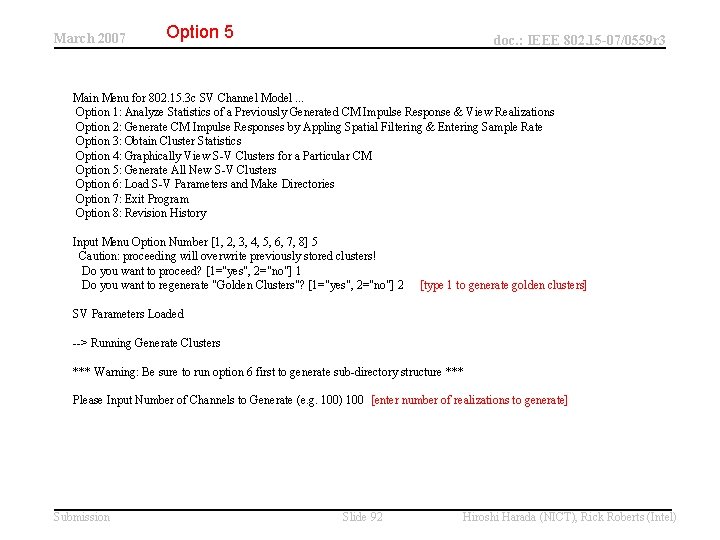
March 2007 Option 5 doc. : IEEE 802. 15 -07/0559 r 3 Main Menu for 802. 15. 3 c SV Channel Model. . . Option 1: Analyze Statistics of a Previously Generated CM Impulse Response & View Realizations Option 2: Generate CM Impulse Responses by Appling Spatial Filtering & Entering Sample Rate Option 3: Obtain Cluster Statistics Option 4: Graphically View S-V Clusters for a Particular CM Option 5: Generate All New S-V Clusters Option 6: Load S-V Parameters and Make Directories Option 7: Exit Program Option 8: Revision History Input Menu Option Number [1, 2, 3, 4, 5, 6, 7, 8] 5 Caution: proceeding will overwrite previously stored clusters! Do you want to proceed? [1="yes", 2="no"] 1 Do you want to regenerate "Golden Clusters"? [1="yes", 2="no"] 2 [type 1 to generate golden clusters] SV Parameters Loaded --> Running Generate Clusters *** Warning: Be sure to run option 6 first to generate sub-directory structure *** Please Input Number of Channels to Generate (e. g. 100) 100 [enter number of realizations to generate] Submission Slide 92 Hiroshi Harada (NICT), Rick Roberts (Intel)

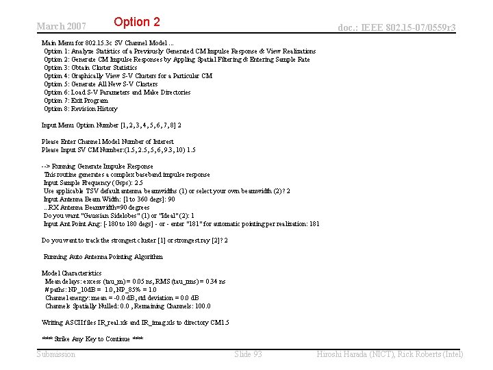
March 2007 Option 2 doc. : IEEE 802. 15 -07/0559 r 3 Main Menu for 802. 15. 3 c SV Channel Model. . . Option 1: Analyze Statistics of a Previously Generated CM Impulse Response & View Realizations Option 2: Generate CM Impulse Responses by Appling Spatial Filtering & Entering Sample Rate Option 3: Obtain Cluster Statistics Option 4: Graphically View S-V Clusters for a Particular CM Option 5: Generate All New S-V Clusters Option 6: Load S-V Parameters and Make Directories Option 7: Exit Program Option 8: Revision History Input Menu Option Number [1, 2, 3, 4, 5, 6, 7, 8] 2 Please Enter Channel Model Number of Interest Please Input SV CM Number: (1. 5, 2. 5, 5, 6, 9. 3, 10) 1. 5 --> Running Generate Impulse Response This routine generates a complex baseband impulse response Input Sample Frequency (Gsps): 2. 5 Use applicable TSV default antenna beamwidths (1) or select your own beamwidth (2)? 2 Input Antenna Beam Width: [1 to 360 degs]: 90. . . RX Antenna Beamwidth=90 degrees Do you want "Gaussian Sidelobes" (1) or "Ideal" (2): 1 Input Ant Point Ang: [-180 to 180 degs] - or - enter "181" for automatic pointing per realization: 181 Do you want to track the strongest cluster [1] or strongest ray [2]? 2 Running Auto Antenna Pointing Algorithm Model Characteristics Mean delays: excess (tau_m) = 0. 05 ns, RMS (tau_rms) = 0. 34 ns # paths: NP_10 d. B = 1. 0, NP_85% = 1. 0 Channel energy: mean = -0. 0 d. B, std deviation = 0. 0 d. B Channels Spatially Nulled: 0. 0 , Remaining Channels: 100. 0 Writing ASCII files IR_real. xls and IR_imag. xls to directory CM 1. 5 *** Strike Any Key to Continue *** Submission Slide 93 Hiroshi Harada (NICT), Rick Roberts (Intel)

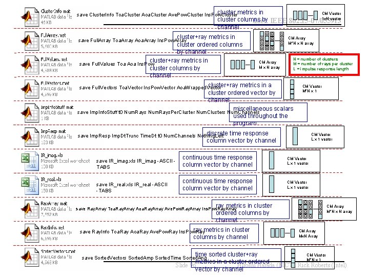
March 2007 doc. : IEEE 802. 15 -07/0559 r 3 CM MAT File Definition Submission Slide 94 Hiroshi Harada (NICT), Rick Roberts (Intel)

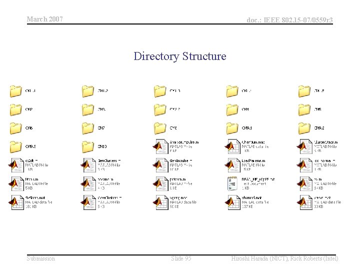
March 2007 doc. : IEEE 802. 15 -07/0559 r 3 Directory Structure Submission Slide 95 Hiroshi Harada (NICT), Rick Roberts (Intel)

March 2007 cluster metrics save Cluster. Info Toa. Cluster Ave. Pow. Cluster Ins. Pow. Cluster in CM Vector 1 x. N vector cluster columns by doc. : IEEE 802. 15 -07/0559 r 3 channel cluster+ray metrics in cluster ordered columns by channel cluster+ray metrics in save Full. Values Toa Aoa Ins. Pow cluster columns by channel save Full. Array Toa. Array Aoa. Array Ins. Pow. Array 0 0 0 CM Array M*N x N array N = number of clusters M = number of rays per cluster L = impulse response length CM Array M x N array cluster+ray save Full. Vectors Toa. Vector Ins. Pow. Vector Aoa. Wrapped. Vector metrics in a cluster ordered vector by channel miscellaneous scalars save Imp. Info. Stuff t 0 Num. Rays. Per. Cluster Num. Clusters Num. Channels used throughout the program CM Vector M*N x 1 discrete save Imp. Resp Imp. Dt. Trunc Time. Dt t 0 Num. Channels Nothing. Left time response column vector by channel save IR_imag. xls IR_imag -ASCII TABS continuous time response column vector by channel CM Vector L x 1 vector save IR_real. xls IR_real -ASCII -TABS continuous time response column vector by channel CM Vector L x 1 vector ray metrics in cluster ordered columns by channel save Ray. Array Toa. Ray. Array Ave. Pow. Ray. Array Ins. Pow. Ray. Array metrics save Ray. Info Toa. Ray Ave. Pow. Ray Ins. Pow. Ray in cluster columns by channel 0 0 0 CM Array M*N x N array CM Array Mx. N Array CM Vector time sorted cluster+ray M*N x 1 metrics in a cluster ordered Slide 96 Hiroshi Harada (NICT), Rick Roberts (Intel) vector by channel save Sorted. Vectors Sorted. Amp Sorted. Time Sorted. Ang Submission CM Vector L x 1 vector

March 2007 doc. : IEEE 802. 15 -07/0559 r 3 SV Flow Chart Submission Slide 97 Hiroshi Harada (NICT), Rick Roberts (Intel)

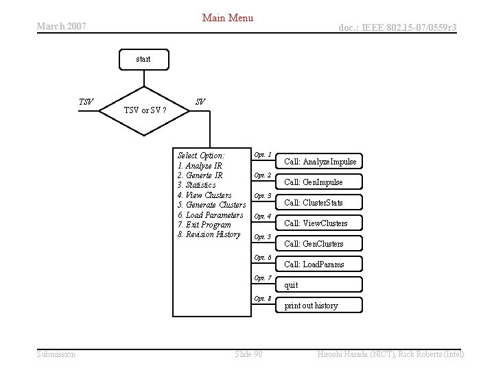
Main Menu March 2007 doc. : IEEE 802. 15 -07/0559 r 3 start TSV or SV ? SV Select Option: 1. Analyze IR 2. Generte IR 3. Statistics 4. View Clusters 5. Generate Clusters 6. Load Parameters 7. Exit Program 8. Revision History Opt. 1 Opt. 2 Opt. 3 Opt. 4 Opt. 5 Opt. 6 Opt. 7 Opt. 8 Submission Slide 98 Call: Analyze. Impulse Call: Gen. Impulse Call: Cluster. Stats Call: View. Clusters Call: Gen. Clusters Call: Load. Params quit print out history Hiroshi Harada (NICT), Rick Roberts (Intel)

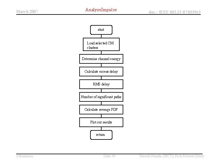
March 2007 Analyze. Impulse doc. : IEEE 802. 15 -07/0559 r 3 start Load selected CM clusters Determine channel energy Calculate excess delay RMS delay Number of significant paths Calculate average PDP Plot out results return Submission Slide 99 Hiroshi Harada (NICT), Rick Roberts (Intel)

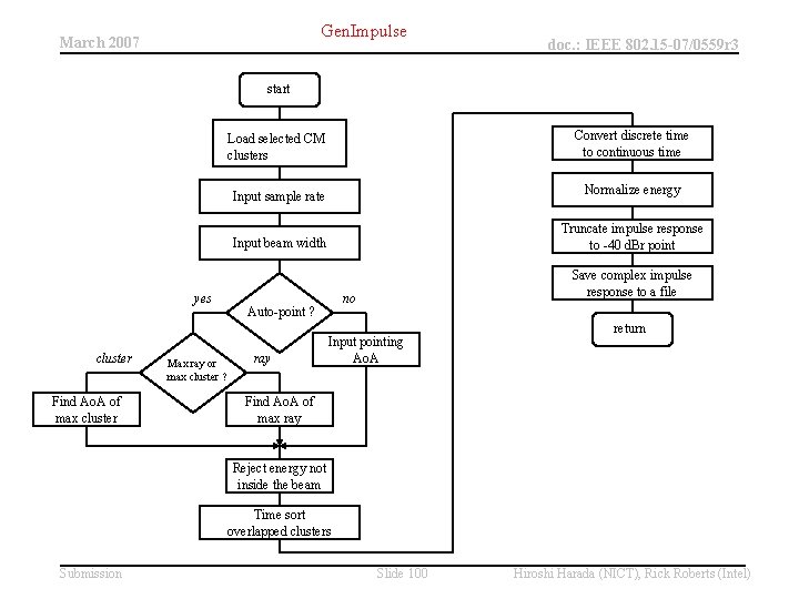
Gen. Impulse March 2007 doc. : IEEE 802. 15 -07/0559 r 3 start yes cluster Find Ao. A of max cluster Max ray or max cluster ? Load selected CM clusters Convert discrete time to continuous time Input sample rate Normalize energy Input beam width Truncate impulse response to -40 d. Br point no Auto-point ? ray Save complex impulse response to a file Input pointing Ao. A return Find Ao. A of max ray Reject energy not inside the beam Time sort overlapped clusters Submission Slide 100 Hiroshi Harada (NICT), Rick Roberts (Intel)

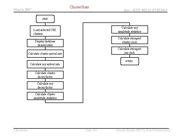
Cluster. Stats March 2007 doc. : IEEE 802. 15 -07/0559 r 3 start Calculate ray amplitude statistics Load selected CM clusters Calculate strongest cluster Ao. A Display database desired stats Calculate strongest ray Ao. A Calculate cluster arrival rate return Calculate ray arrival rate Calculate cluster decay factor Calculate ray decay factor Calculate cluster amplitude statistics Submission Slide 101 Hiroshi Harada (NICT), Rick Roberts (Intel)

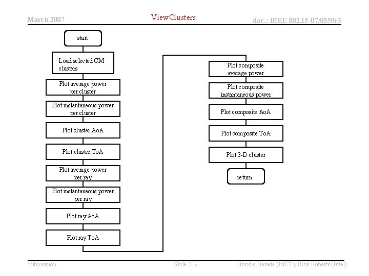
View. Clusters March 2007 doc. : IEEE 802. 15 -07/0559 r 3 start Load selected CM clusters Plot composite average power Plot average power per cluster Plot composite instantaneous power Plot instantaneous power per cluster Plot composite Ao. A Plot cluster Ao. A Plot composite To. A Plot cluster To. A Plot 3 -D cluster Plot average power per ray return Plot instantaneous power per ray Plot ray Ao. A Plot ray To. A Submission Slide 102 Hiroshi Harada (NICT), Rick Roberts (Intel)

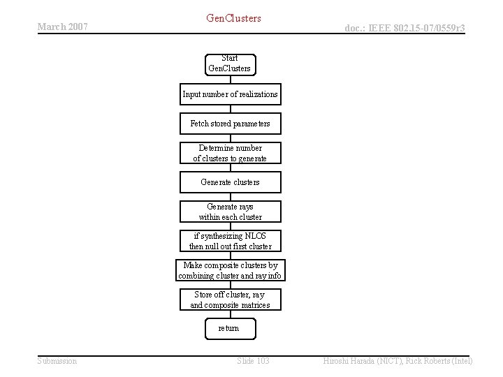
March 2007 Gen. Clusters doc. : IEEE 802. 15 -07/0559 r 3 Start Gen. Clusters Input number of realizations Fetch stored parameters Determine number of clusters to generate Generate clusters Generate rays within each cluster if synthesizing NLOS then null out first cluster Make composite clusters by combining cluster and ray info Store off cluster, ray and composite matrices return Submission Slide 103 Hiroshi Harada (NICT), Rick Roberts (Intel)

March 2007 doc. : IEEE 802. 15 -07/0559 r 3 Open issue in Jan. 16 2007 and comments p CM 1. 5 is missing in the MATLAB code – The version 1. 1 code includes the missing CM in the flow of TSV model. p How beam-width of RX antenna changes? – You can input the beam-width from Menu. m in Ver 1. 1 code p Does the code do any limitation if power of ray before the multiplication by antenna gain is higher than free space loss + 6 d. B ? – No, the code does not use any limitation. p When changed beam-width of TX antenna, why the number of rays did not decrease ? – This is a channel model issue not MATLAB code issue p For CM 2 and CM 4, how to steer the direction of antenna – The direction to antenna is that to get maximum total power. Version 1. 1 does not include the model. Next version will include it. The modified code will be released by Jan. 31 (in TSV flow) – In the version 1. 1, the two antennas are faced to each other. p When Version 1. 1 is released? – On Jan. 16 the code will be released Submission Slide 104 Hiroshi Harada (NICT), Rick Roberts (Intel)