Introduction to NGS Data Analysis Group 2 nd

Introduction to NGS Data Analysis Group 2 nd August 2019 http: //dag. compbio. dundee. ac. uk cb-dag@dundee. ac. uk @Uo. D_DAG

Outline • Sequencing history • Current sequencing approaches • File formats • Quality assessment • Read trimming • DAG workflows • The Sequence Read Archive

Key to slides…. • Descriptive text • Example commands – black monospaced text: ls /tmp • Commands to run – red monospaced text • Prompts/STDOUT/STDERR – green monospaced text • e. g. -bash-4. 1 $ echo $USER jabbott • [ENTER] – press enter key • [username] – your username, not '[username]' • - command is continued on next line – don't press 'enter' at this point

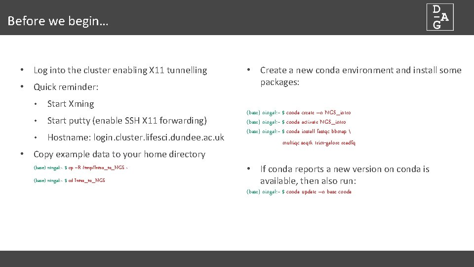
Before we begin… • Log into the cluster enabling X 11 tunnelling • Quick reminder: • Start Xming • Start putty (enable SSH X 11 forwarding) • Hostname: login. cluster. lifesci. dundee. ac. uk • Copy example data to your home directory (base) ningal: ~ $ cp –R /tmp/Intro_to_NGS ~ (base) ningal: ~ $ cd Intro_to_NGS • Create a new conda environment and install some packages: (base) ningal: ~ $ conda create –n NGS_intro (base) ningal: ~ $ conda activate NGS_intro (base) ningal: ~ $ conda install fastqc bbmap multiqc seqtk trim-galore readfq • If conda reports a new version on conda is available, then also run: (base) ningal: ~ $ conda update –n base conda

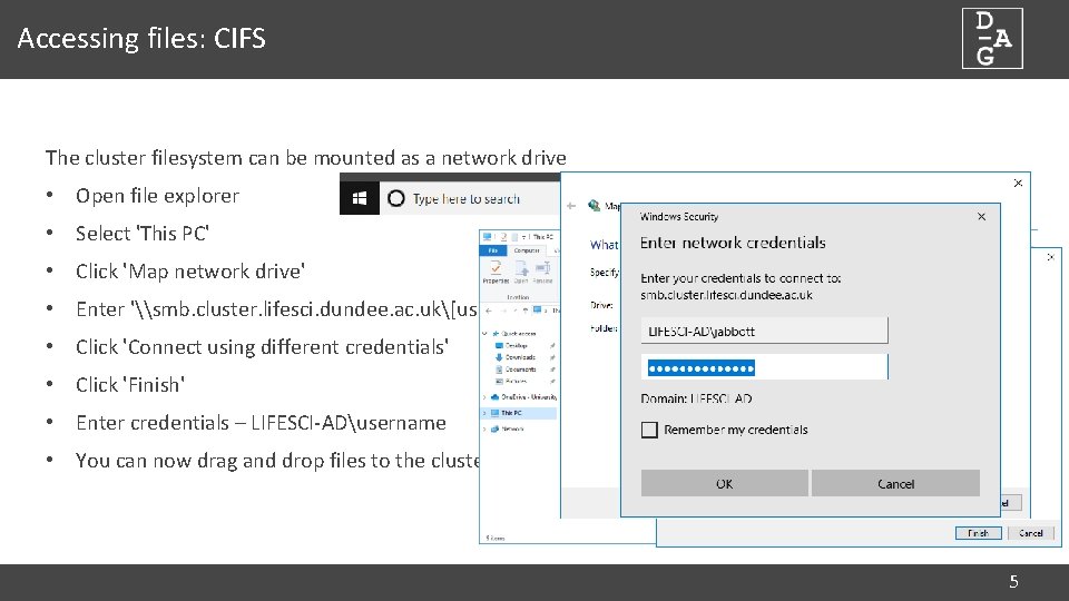
Accessing files: CIFS The cluster filesystem can be mounted as a network drive • Open file explorer • Select 'This PC' • Click 'Map network drive' • Enter '\smb. cluster. lifesci. dundee. ac. uk[username] • Click 'Connect using different credentials' • Click 'Finish' • Enter credentials – LIFESCI-ADusername • You can now drag and drop files to the cluster 5

An Abridged History of Sequencing dundee. ac. uk http: //dag. compbio. dundee. ac. uk cb-dag@dundee. ac. uk @Uo. D_DAG Page

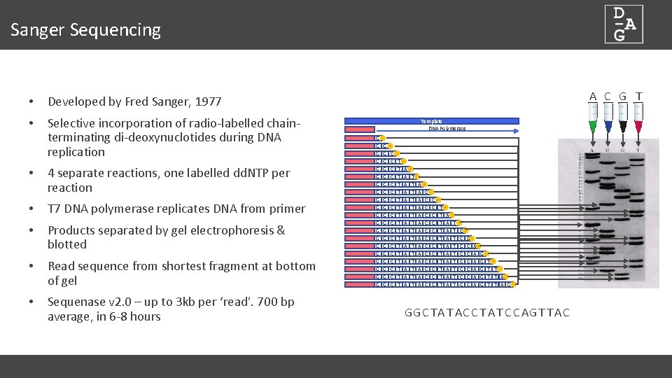
Sanger Sequencing • Developed by Fred Sanger, 1977 • Selective incorporation of radio-labelled chainterminating di-deoxynuclotides during DNA replication • 4 separate reactions, one labelled dd. NTP per reaction • T 7 DNA polymerase replicates DNA from primer • Products separated by gel electrophoresis & blotted • Read sequence from shortest fragment at bottom of gel • Sequenase v 2. 0 – up to 3 kb per ‘read’. 700 bp average, in 6 -8 hours A C G T Template DNA Polymerase G G G G G G G G G G C C C C C T T T T T A A A A T T T T A A A A C C C C C C C T T T A A A A A T T T T T C C C C A A A G G G T T T A C GGC TA T AC C T A T C C AG T T AC

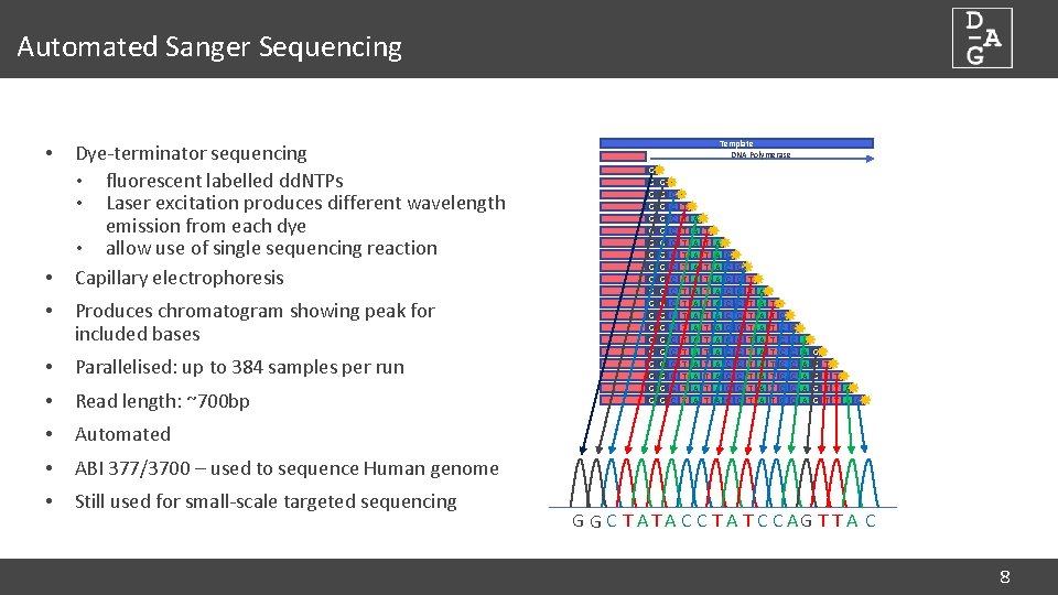
Automated Sanger Sequencing • • • Dye-terminator sequencing • fluorescent labelled dd. NTPs • Laser excitation produces different wavelength emission from each dye • allow use of single sequencing reaction Capillary electrophoresis Produces chromatogram showing peak for included bases • Parallelised: up to 384 samples per run • Read length: ~700 bp • Automated • ABI 377/3700 – used to sequence Human genome • Still used for small-scale targeted sequencing Template DNA Polymerase G G G G G G G G G G C C C C C T T T T T A A A A T T T T A A A A C C C C C C C T T T A A A A A T T T T T C C C C A A A G G G T T T A C G G C T A C C T A T C C AG T T A C 8

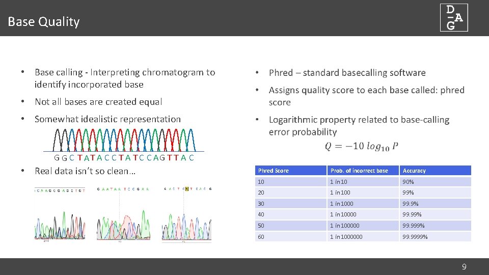
Base Quality • Base calling - Interpreting chromatogram to identify incorporated base • Not all bases are created equal • Somewhat idealistic representation G G C T A C C T A T C C AG T T A C • Real data isn’t so clean… Phred Score Prob. of incorrect base Accuracy 10 1 in 10 90% 20 1 in 100 99% 30 1 in 1000 99. 9% 40 1 in 10000 99. 99% 50 1 in 100000 99. 999% 60 1 in 1000000 99. 9999% 9

Current Sequencing Approaches dundee. ac. uk http: //dag. compbio. dundee. ac. uk cb-dag@dundee. ac. uk @Uo. D_DAG Page

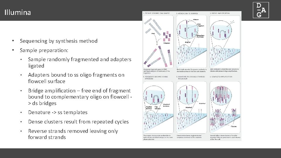
Illumina • Sequencing by synthesis method • Sample preparation: • Sample randomly fragmented and adapters ligated • Adapters bound to ss oligo fragments on flowcell surface • Bridge amplification – free end of fragment bound to complementary oligo on flowcell > ds bridges • Denature -> ss templates • Dense clusters result from repeated cycles • Reverse strands removed leaving only forward strands

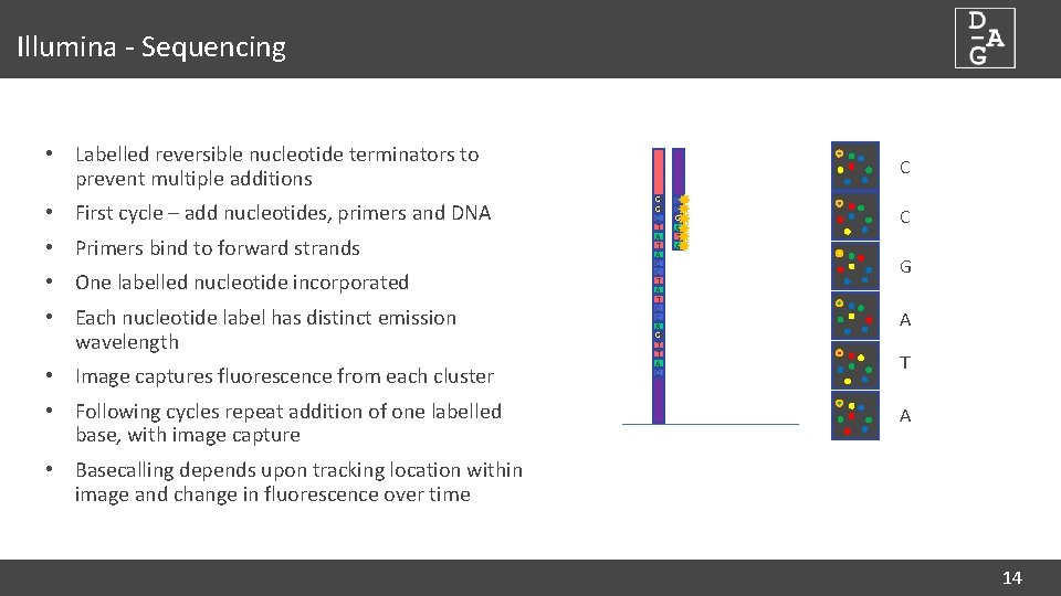
Illumina - Sequencing • Labelled reversible nucleotide terminators to prevent multiple additions • First cycle – add nucleotides, primers and DNA • Primers bind to forward strands • One labelled nucleotide incorporated • Each nucleotide label has distinct emission wavelength • Image captures fluorescence from each cluster • Following cycles repeat addition of one labelled base, with image capture C G G C T A C C T A T C C A G T T A C C C G A T A • Basecalling depends upon tracking location within image and change in fluorescence over time 14

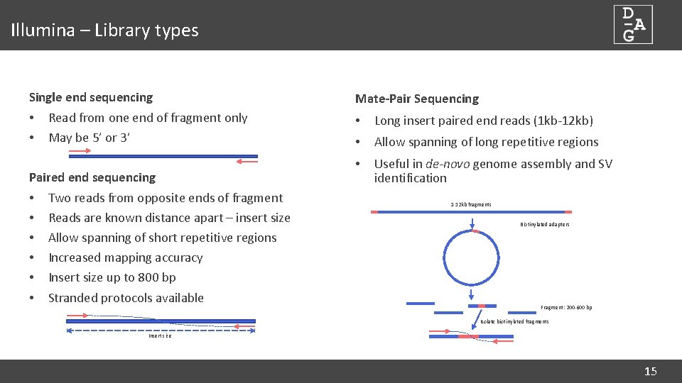
Illumina – Library types Single end sequencing • Read from one end of fragment only • May be 5’ or 3’ Paired end sequencing • Two reads from opposite ends of fragment • Reads are known distance apart – insert size • Allow spanning of short repetitive regions • Increased mapping accuracy • Insert size up to 800 bp • Stranded protocols available Mate-Pair Sequencing • Long insert paired end reads (1 kb-12 kb) • Allow spanning of long repetitive regions • Useful in de-novo genome assembly and SV identification 2 -12 kb fragments Biotinylated adapters Fragment: 200 -600 bp Isolate biotinylated fragments Insert size 15

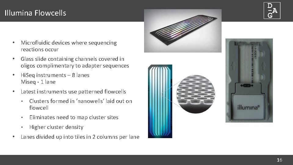
Illumina Flowcells • Microfluidic devices where sequencing reactions occur • Glass slide containing channels covered in oligos complimentary to adapter sequences • Hi. Seq instruments – 8 lanes Miseq - 1 lane • Latest instruments use patterned flowcells • Clusters formed in ‘nanowells’ laid out on flowcell • Eliminates need to map cluster sites • Higher cluster density • Lanes divided up into tiles in 2 columns per lane 16

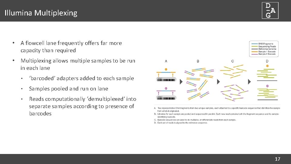
Illumina Multiplexing • A flowcell lane frequently offers far more capacity than required • Multiplexing allows multiple samples to be run in each lane • ‘barcoded’ adapters added to each sample • Samples pooled and run on lane • Reads computationally ‘demultiplexed’ into separate samples according to presence of barcodes 17

Long Read Technologies • Short read sequencing produces vast data volumes • Backward step compared to Sanger sequencing • De-novo assembly limited • RNA sequencing – splice detection harder • SV detection more difficult • Long reads generated from single molecules help • Resolve repeats in de-novo assembly • Sequence entire RNA molecules to reveal splicing • Aid SV identification • Downsides • High error rates 18

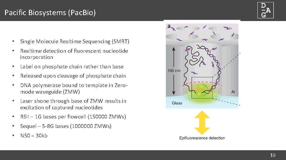
Pacific Biosystems (Pac. Bio) • Single Molecule Realtime Sequencing (SMRT) • Realtime detection of fluorescent nucleotide incorporation • Label on phosphate chain rather than base • Released upon cleavage of phosphate chain • DNA polymerase bound to template in Zeromode waveguide (ZMW) • Laser shone through base of ZMW results in excitation of captured nucleotides • RSII – 1 G bases per flowcell (150000 ZMWs) • Sequel – 5 -8 G bases (1000000 ZMWs) • N 50 = 30 kb 19

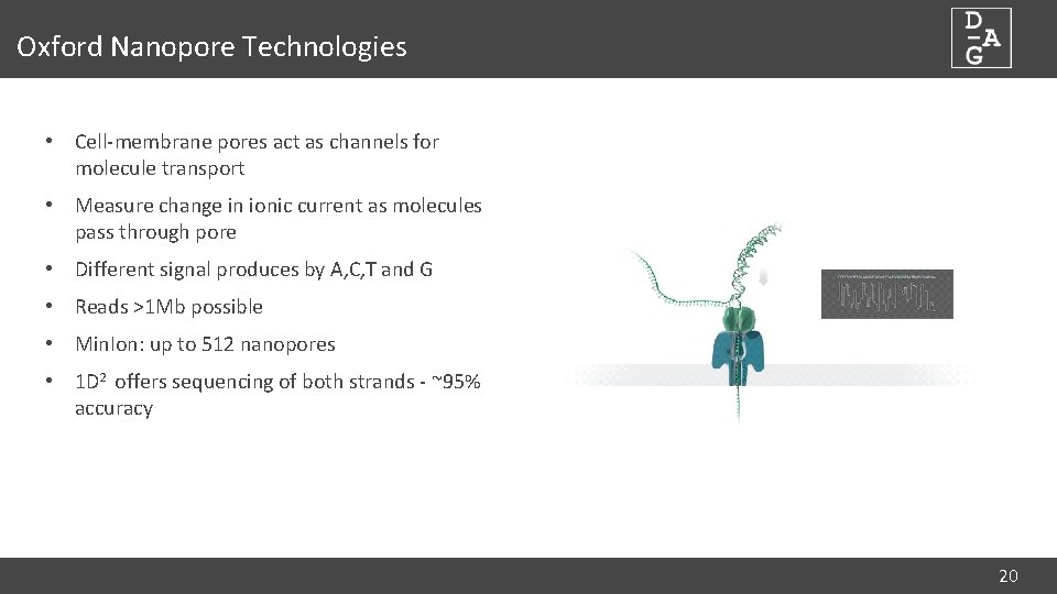
Oxford Nanopore Technologies • Cell-membrane pores act as channels for molecule transport • Measure change in ionic current as molecules pass through pore • Different signal produces by A, C, T and G • Reads >1 Mb possible • Min. Ion: up to 512 nanopores • 1 D 2 offers sequencing of both strands - ~95% accuracy 20

File Formats dundee. ac. uk http: //dag. compbio. dundee. ac. uk cb-dag@dundee. ac. uk @Uo. D_DAG Page

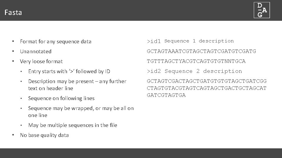
Fasta • Format for any sequence data >id 1 Sequence 1 description • Unannotated GCTAGTAAATCGTAGCTAGTCGATG • Very loose format TGTTTAGCTYACGTCAGTGTGTNNTGCA • Entry starts with ‘>’ followed by ID >id 2 Sequence 2 description • Description may be present – any further text on header line • Sequence on following lines GCTAGTCGACTAGCTGATGTGTGTAGCTGATCGG CTAGTGTACGTAGTCAGTAGCTGACTGCTAGCAT GATCGTAGTGA • Sequence may be wrapped, or may be all on one line • May be multiple sequences in the file • No base quality data

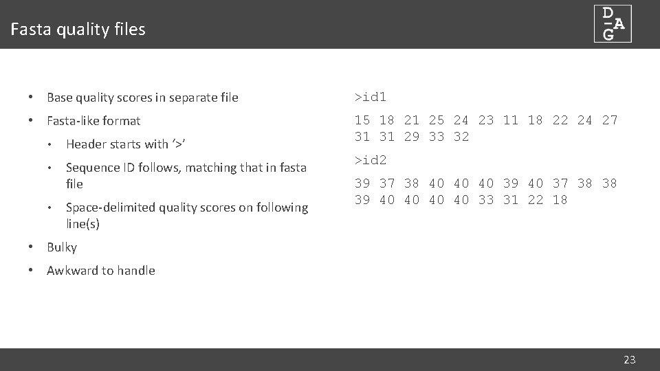
Fasta quality files • Base quality scores in separate file >id 1 • Fasta-like format 15 18 21 25 24 23 11 18 22 24 27 31 31 29 33 32 • Header starts with ‘>’ • Sequence ID follows, matching that in fasta file • Space-delimited quality scores on following line(s) >id 2 39 37 38 40 40 40 39 40 37 38 38 39 40 40 33 31 22 18 • Bulky • Awkward to handle 23

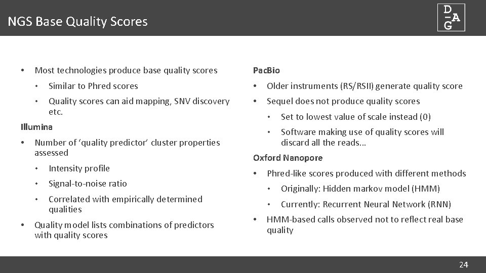
NGS Base Quality Scores • Most technologies produce base quality scores Pac. Bio • Similar to Phred scores • Older instruments (RS/RSII) generate quality score • Quality scores can aid mapping, SNV discovery etc. • Sequel does not produce quality scores Illumina • • Number of ‘quality predictor’ cluster properties assessed • Intensity profile • Signal-to-noise ratio • Correlated with empirically determined qualities Quality model lists combinations of predictors with quality scores • Set to lowest value of scale instead (0) • Software making use of quality scores will discard all the reads… Oxford Nanopore • • Phred-like scores produced with different methods • Originally: Hidden markov model (HMM) • Currently: Recurrent Neural Network (RNN) HMM-based calls observed not to reflect real base quality 24

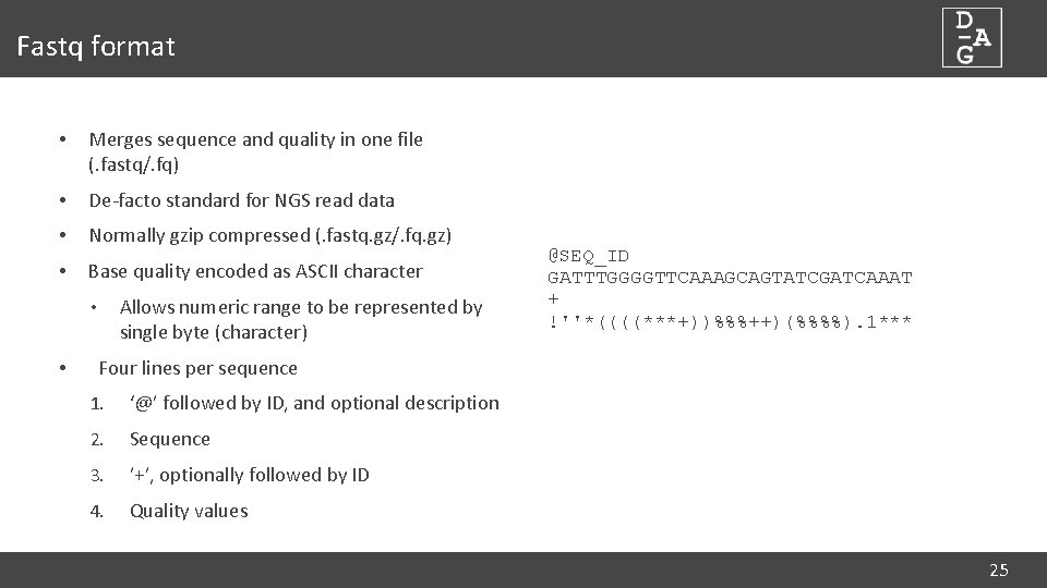
Fastq format • Merges sequence and quality in one file (. fastq/. fq) • De-facto standard for NGS read data • Normally gzip compressed (. fastq. gz/. fq. gz) • Base quality encoded as ASCII character Allows numeric range to be represented by single byte (character) • • @SEQ_ID GATTTGGGGTTCAAAGCAGTATCGATCAAAT + !''*((((***+))%%%++)(%%%%). 1*** Four lines per sequence 1. ‘@’ followed by ID, and optional description 2. Sequence 3. ’+’, optionally followed by ID 4. Quality values 25

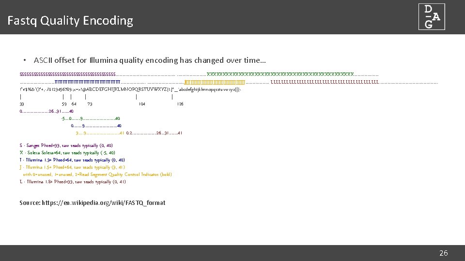
Fastq Quality Encoding • ASCII offset for Illumina quality encoding has changed over time… SSSSSSSSSSSSSSSSSSSSS. . . . . XXXXXXXXXXXXXXXXXXXXXXX. . . . IIIIIIIIIIIIIIIIIIIII. . . . JJJJJJJJJJJJJJJJJJJJ. . . . . LLLLLLLLLLLLLLLLLLLLL. . . . !"#$%&'()*+, -. /0123456789: ; <=>? @ABCDEFGHIJKLMNOPQRSTUVWXYZ[]^_`abcdefghijklmnopqrstuvwxyz{|}~ | | | 33 59 64 73 104 126 0. . . 26. . . 31. . . . 40 -5. . 0. . . . 9. . . . 40 3. . . 9. . . . 41 0. 2. . . . . 26. . . 31. . . . 41 S - Sanger Phred+33, raw reads typically (0, 40) X - Solexa+64, raw reads typically (-5, 40) I - Illumina 1. 3+ Phred+64, raw reads typically (0, 40) J - Illumina 1. 5+ Phred+64, raw reads typically (3, 41) with 0=unused, 1=unused, 2=Read Segment Quality Control Indicator (bold) L - Illumina 1. 8+ Phred+33, raw reads typically (0, 41) Source: https: //en. wikipedia. org/wiki/FASTQ_format 26

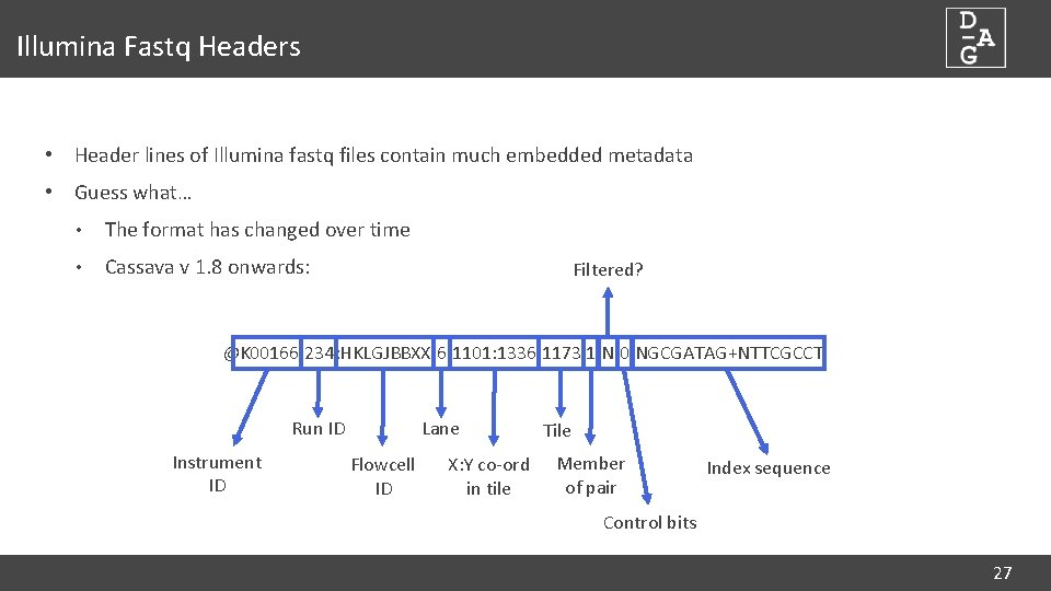
Illumina Fastq Headers • Header lines of Illumina fastq files contain much embedded metadata • Guess what… • The format has changed over time • Cassava v 1. 8 onwards: Filtered? @K 00166: 234: HKLGJBBXX: 6: 1101: 1336: 1173 1: N: 0: NGCGATAG+NTTCGCCT Run ID Instrument ID Lane Flowcell ID X: Y co-ord in tile Tile Member of pair Index sequence Control bits 27

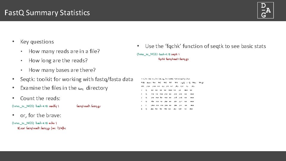
Fast. Q Summary Statistics • Key questions • How many reads are in a file? • How long are the reads? • How many bases are there? • Seqtk: toolkit for working with fastq/fasta data • Examine the files in the fastq directory • Count the reads: (Intro_to_NGS) -bash-4. 1$ readfq • or, for the brave: (Intro_to_NGS) -bash-4. 1$ echo $(zcat fastq/read 1. fastq. gz |wc -l)/4|bc fastq/read 1. fastq. gz • Use the ‘fqchk’ function of seqtk to see basic stats (Intro_to_NGS) -bash-4. 1$ seqtk fqchk fastq/read 1. fastq. gz min_len: 150; max_len: 150; avg_len: 150. 00; 7 distinct quality values POS #bases %A ALL 3750 %C %G %T 34. 6 14. 2 13. 3 37. 2 0. 7 %N avg. Q err. Q %low 38. 5 23. 2 3. 0 2. 5 97. 5 1 25 0. 0 100. 0 2 25 44. 0 20. 0 32. 0 100. 0 3 25 32. 0 20. 0 8. 0 40. 0 31. 8 31. 6 0. 0 100. 0 4 25 48. 0 12. 0 4. 0 36. 0 0. 0 36. 2 35. 7 0. 0 100. 0 5 2 520. 0 12. 0 56. 0 0. 0 36. 0 34. 4 0. 0 100. 0 6 25 36. 0. 8. 0 48. 0 0. 0 39. 3 25. 8 4. 0 96. 0 %high

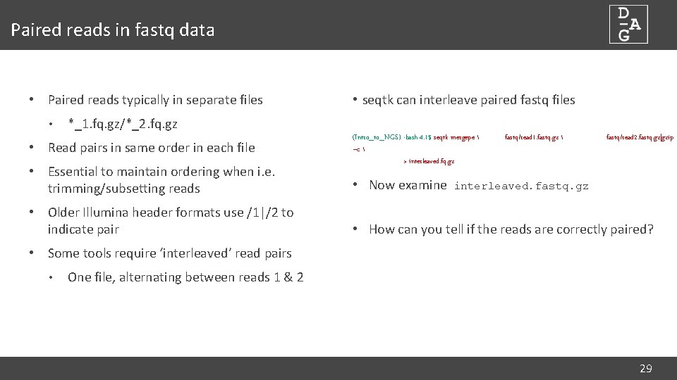
Paired reads in fastq data • Paired reads typically in separate files • • seqtk can interleave paired fastq files *_1. fq. gz/*_2. fq. gz • Read pairs in same order in each file • Essential to maintain ordering when i. e. trimming/subsetting reads • Older Illumina header formats use /1|/2 to indicate pair (Intro_to_NGS) -bash-4. 1$ seqtk mergepe –c > interleaved. fq. gz • Now examine fastq/read 1. fastq. gz fastq/read 2. fastq. gz|gzip interleaved. fastq. gz • How can you tell if the reads are correctly paired? • Some tools require ‘interleaved’ read pairs • One file, alternating between reads 1 & 2 29

Quality Assessment dundee. ac. uk http: //dag. compbio. dundee. ac. uk cb-dag@dundee. ac. uk @Uo. D_DAG Page

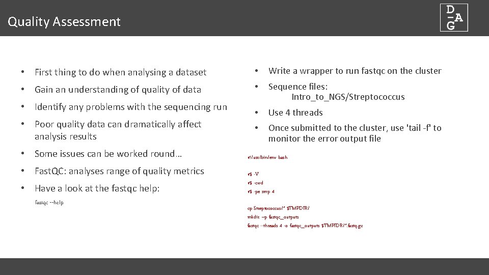
Quality Assessment • First thing to do when analysing a dataset • Write a wrapper to run fastqc on the cluster • Gain an understanding of quality of data • • Identify any problems with the sequencing run Sequence files: Intro_to_NGS/Streptococcus • Use 4 threads • Once submitted to the cluster, use 'tail -f' to monitor the error output file • Poor quality data can dramatically affect analysis results • Some issues can be worked round… • Fast. QC: analyses range of quality metrics • Have a look at the fastqc help: fastqc --help #!/usr/bin/env bash #$ -V #$ -cwd #$ -pe smp 4 cp Streptococcus/* $TMPDIR/ mkdir –p fastqc_outputs fastqc --threads 4 -o fastqc_outputs $TMPIDR/*. fastq. gz

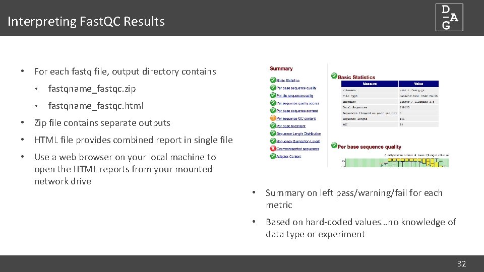
Interpreting Fast. QC Results • For each fastq file, output directory contains • fastqname_fastqc. zip • fastqname_fastqc. html • Zip file contains separate outputs • HTML file provides combined report in single file • Use a web browser on your local machine to open the HTML reports from your mounted network drive • Summary on left pass/warning/fail for each metric • Based on hard-coded values…no knowledge of data type or experiment 32

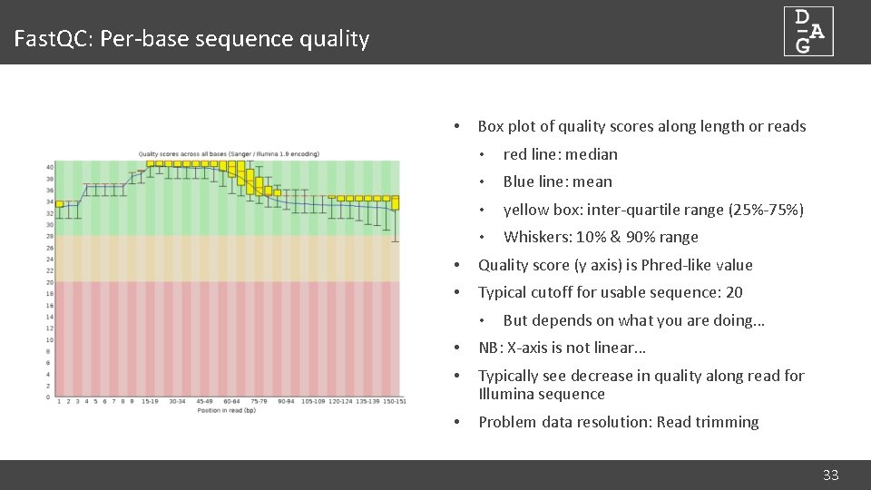
Fast. QC: Per-base sequence quality • Box plot of quality scores along length or reads • red line: median • Blue line: mean • yellow box: inter-quartile range (25%-75%) • Whiskers: 10% & 90% range • Quality score (y axis) is Phred-like value • Typical cutoff for usable sequence: 20 • But depends on what you are doing… • NB: X-axis is not linear… • Typically see decrease in quality along read for Illumina sequence • Problem data resolution: Read trimming 33

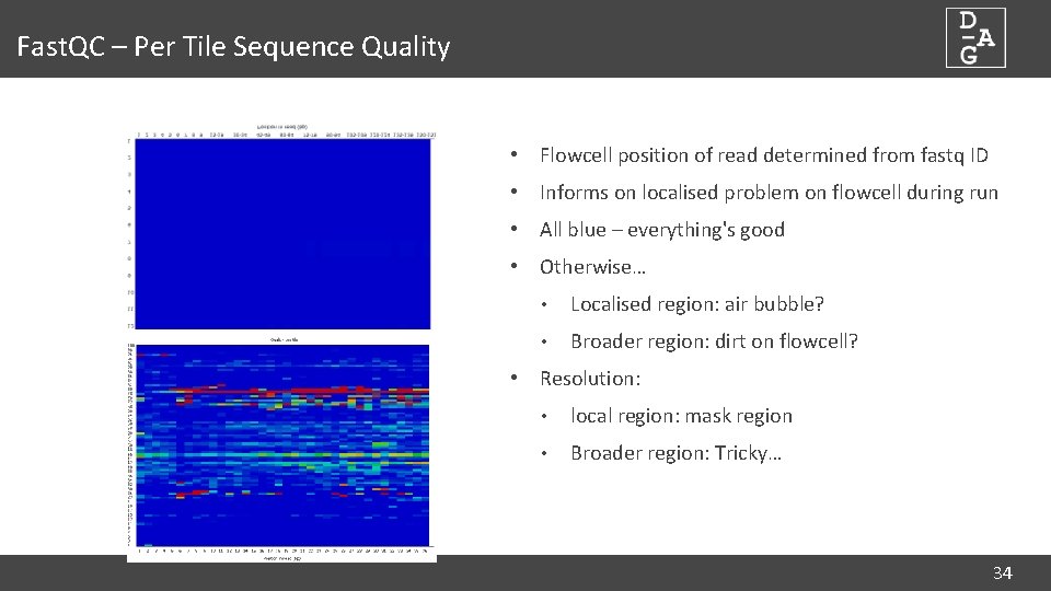
Fast. QC – Per Tile Sequence Quality • Flowcell position of read determined from fastq ID • Informs on localised problem on flowcell during run • All blue – everything's good • Otherwise… • Localised region: air bubble? • Broader region: dirt on flowcell? • Resolution: • local region: mask region • Broader region: Tricky… 34

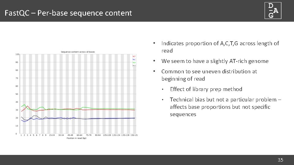
Fast. QC – Per-base sequence content • Indicates proportion of A, C, T, G across length of read • We seem to have a slightly AT-rich genome • Common to see uneven distribution at beginning of read • Effect of library prep method • Technical bias but not a particular problem – affects base proportions but not specific sequences 35

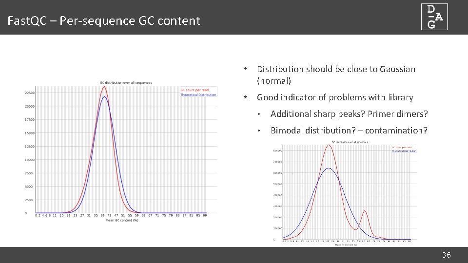
Fast. QC – Per-sequence GC content • Distribution should be close to Gaussian (normal) • Good indicator of problems with library • Additional sharp peaks? Primer dimers? • Bimodal distribution? – contamination? 36

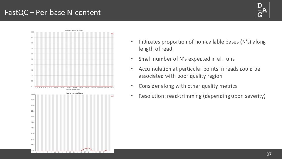
Fast. QC – Per-base N-content • Indicates proportion of non-callable bases (N’s) along length of read • Small number of N’s expected in all runs • Accumulation at particular points in reads could be associated with poor quality region • Consider along with other quality metrics • Resolution: read-trimming (depending upon severity) 37

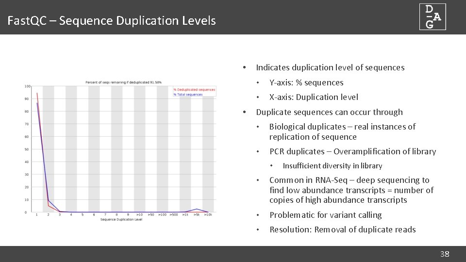
Fast. QC – Sequence Duplication Levels • • Indicates duplication level of sequences • Y-axis: % sequences • X-axis: Duplication level Duplicate sequences can occur through • Biological duplicates – real instances of replication of sequence • PCR duplicates – Overamplification of library • Insufficient diversity in library • Common in RNA-Seq – deep sequencing to find low abundance transcripts = number of copies of high abundance transcripts • Problematic for variant calling • Resolution: Removal of duplicate reads 38

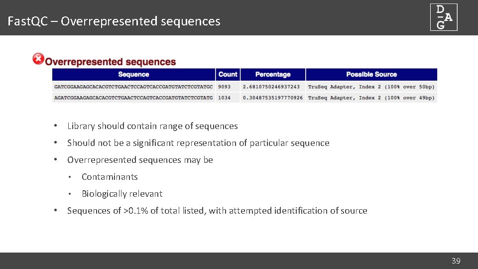
Fast. QC – Overrepresented sequences • Library should contain range of sequences • Should not be a significant representation of particular sequence • Overrepresented sequences may be • Contaminants • Biologically relevant • Sequences of >0. 1% of total listed, with attempted identification of source 39

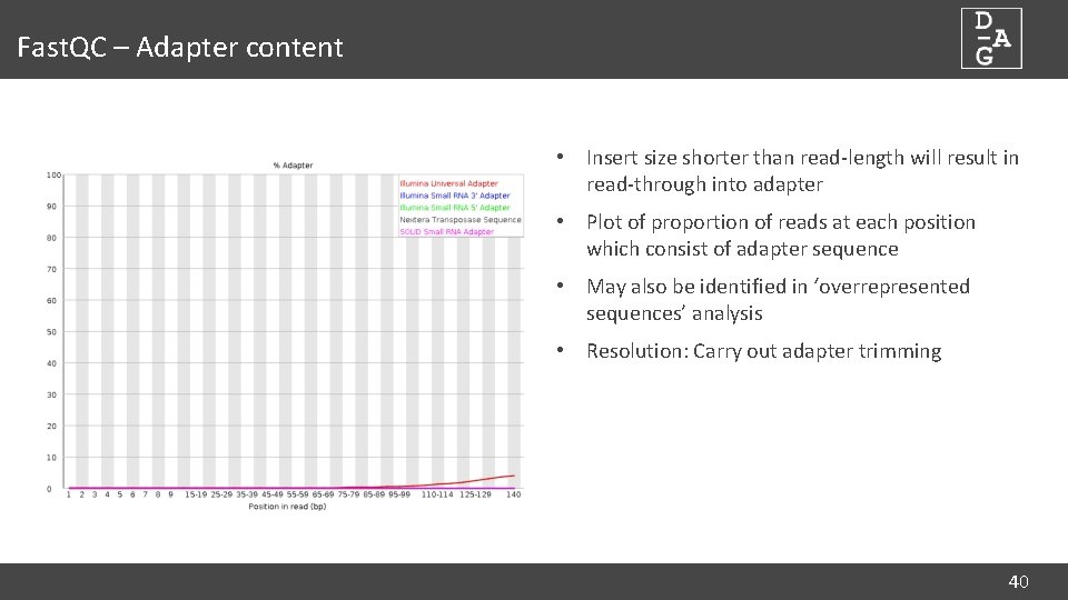
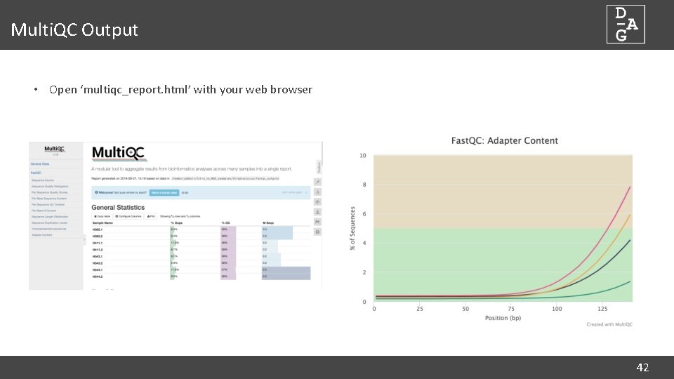
Fast. QC – Adapter content • Insert size shorter than read-length will result in read-through into adapter • Plot of proportion of reads at each position which consist of adapter sequence • May also be identified in ‘overrepresented sequences’ analysis • Resolution: Carry out adapter trimming 40

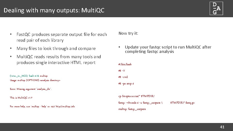
Dealing with many outputs: Multi. QC • Fast. QC produces separate output file for each read pair of each library Now try it: • Many files to look through and compare • • Multi. QC reads results from many tools and produces single interactive HTML report (Intro_to_NGS) -bash-4. 1$ multiqc Usage: multiqc [OPTIONS] <analysis directory> Update your fastqc script to run Multi. QC after completing fastqc analysis #!/bin/bash #$ -V #$ -cwd #$ -pe smp 4 Error: Missing argument "analysis_dir". This is Multi. QC v 1. 7 For more help, run 'multiqc --help' or visit http: //multiqc. info cp Streptococcus/* $TMPDIR/ fastqc --threads 4 -o fastqc_outputs $TMPDIR/*. fastq. gz multiqc fastqc_outputs 41

Multi. QC Output • Open ‘multiqc_report. html’ with your web browser 42

Read Trimming dundee. ac. uk http: //dag. compbio. dundee. ac. uk cb-dag@dundee. ac. uk @Uo. D_DAG Page

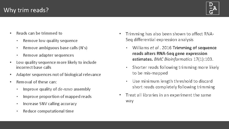
Why trim reads? • Reads can be trimmed to • Remove low quality sequence • Remove ambiguous base calls (N’s) • Remove adapter sequences • Low quality sequence more likely to include incorrect base calls • Adapter sequences not of biological relevance • Removal of these can: • Improve quality of de-novo assembly • Improve proportion of mapped reads • Increase SNV calling accuracy • Reduce computational time • Trimming has also been shown to affect RNASeq differential expression analysis • Williams et al. 2016 Trimming of sequence reads alters RNA-Seq gene expression estimates. BMC Bioinformatics 17(1): 103. • Shorter reads following trimming more likely to be mis-mapped • Use minimum length threshold to discard short reads completely following trimming • Treat all libraries in an experiment the same way

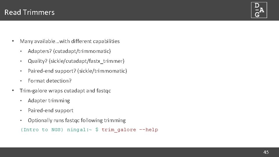
Read Trimmers • Many available…with different capabilities • Adapters? (cutadapt/trimmomatic) • Quality? (sickle/cutadapt/fastx_trimmer) • Paired-end support? (sickle/trimmomatic) • Format detection? • Trim-galore wraps cutadapt and fastqc • Adapter trimming • Paired-end support • Optionally runs fastqc following trimming (Intro to NGS) ningal: ~ $ trim_galore --help 45

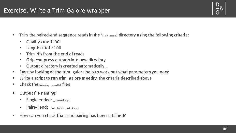
Exercise: Write a Trim Galore wrapper • • • Trim the paired-end sequence reads in the ‘Streptococcus’ directory using the following criteria: • Quality cutoff: 30 • Length cutoff: 100 • Trim N’s from the end of reads • Gzip compress outputs into new directory • Output directory is created automatically… Start by looking at the trim_galore help to work out what parameters you need Write a script to run trim_galore meeting the criteria described above Check the trimming_report. txt files Output file naming: • Single ended: _trimmed. fq. gz • • Paired end: _val_1. fq. gz, _val_2. fq. gz How can you check that read pairing has been retained? 46

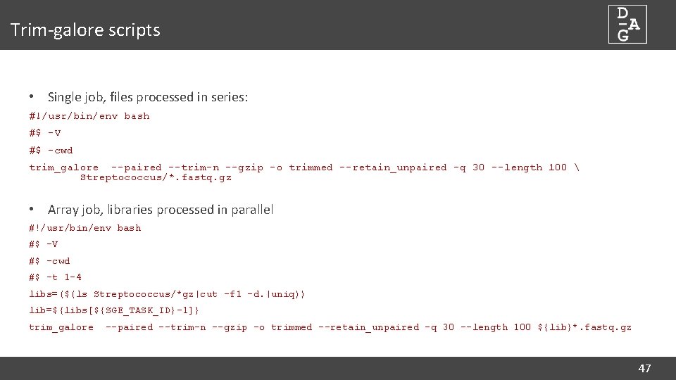
Trim-galore scripts • Single job, files processed in series: #!/usr/bin/env bash #$ -V #$ -cwd trim_galore --paired --trim-n --gzip -o trimmed --retain_unpaired -q 30 --length 100 Streptococcus/*. fastq. gz • Array job, libraries processed in parallel #!/usr/bin/env bash #$ -V #$ -cwd #$ -t 1 -4 libs=($(ls Streptococcus/*gz|cut -f 1 -d. |uniq)) lib=${libs[${SGE_TASK_ID}-1]} trim_galore --paired --trim-n --gzip -o trimmed --retain_unpaired -q 30 --length 100 ${lib}*. fastq. gz 47

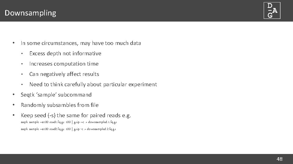
Downsampling • In some circumstances, may have too much data • Excess depth not informative • Increases computation time • Can negatively affect results • Need to think carefully about particular experiment • Seqtk ‘sample’ subcommand • Randomly subsambles from file • Keep seed (-s) the same for paired reads e. g. seqtk sample –s 100 read 1. fq. gz 100 | gzip –c > downsampled. 1. fq. gz seqtk sample –s 100 read 2. fq. gz 100 | gzip -c > downsampled. 2. fq. gz 48

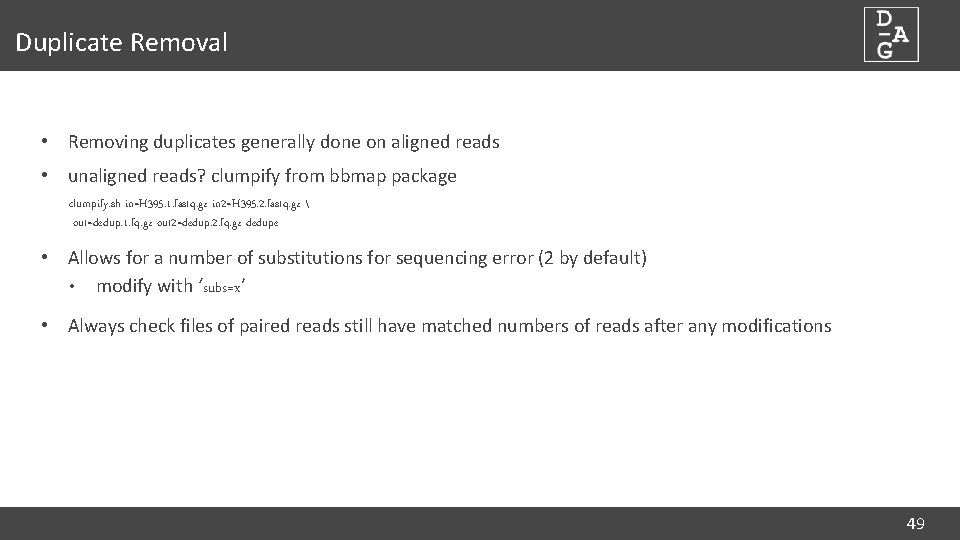
Duplicate Removal • Removing duplicates generally done on aligned reads • unaligned reads? clumpify from bbmap package clumpify. sh in=H 395. 1. fastq. gz in 2=H 395. 2. fastq. gz out=dedup. 1. fq. gz out 2=dedup. 2. fq. gz dedupe • Allows for a number of substitutions for sequencing error (2 by default) • modify with ‘subs=x’ • Always check files of paired reads still have matched numbers of reads after any modifications 49

DAG Workflows dundee. ac. uk http: //dag. compbio. dundee. ac. uk cb-dag@dundee. ac. uk @Uo. D_DAG Page

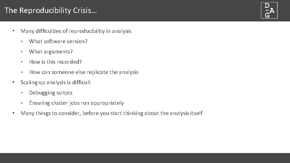
The Reproducibility Crisis… • Many difficulties of reproducibility in analysis • What software version? • What arguments? • How is this recorded? • How can someone else replicate the analysis • Scaling up analysis is difficult • Debugging scripts • Ensuring cluster jobs run appropriately • Many things to consider, before you start thinking about the analysis itself

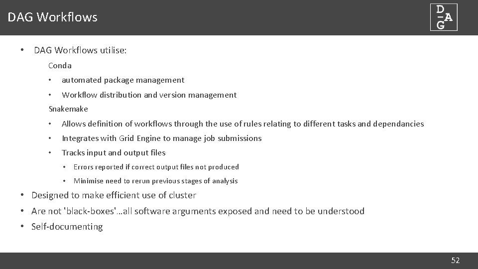
DAG Workflows • DAG Workflows utilise: Conda • automated package management • Workflow distribution and version management Snakemake • Allows definition of workflows through the use of rules relating to different tasks and dependancies • Integrates with Grid Engine to manage job submissions • Tracks input and output files • Errors reported if correct output files not produced • Minimise need to rerun previous stages of analysis • Designed to make efficient use of cluster • Are not 'black-boxes'…all software arguments exposed and need to be understood • Self-documenting 52

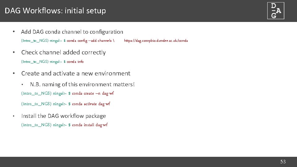
DAG Workflows: initial setup • Add DAG conda channel to configuration (Intro_to_NGS) ningal: ~ $ conda config --add channels • https: //dag. compbio. dundee. ac. uk/conda Check channel added correctly (Intro_to_NGS) ningal: ~ $ conda info • Create and activate a new environment N. B. naming of this environment matters! (Intro_to_NGS) ningal: ~ $ conda create –n dag-wf • (Intro_to_NGS) ningal: ~ $ conda activate dag-wf • Install the DAG workflow package (Intro_to_NGS) ningal: ~ $ conda install dag-wf 53

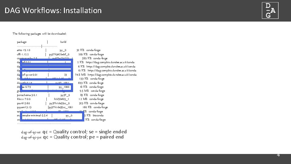
DAG Workflows: Installation The following packages will be downloaded: package | build --------------|--------attrs-19. 1. 0 | py_0 32 KB conda-forge cffi-1. 12. 2 | py 37 h 342 bebf_0 209 KB conda-forge cryptography-2. 5 | py 37 hc 2 b 1221_1 589 KB conda-forge dag-wf-0. 01 | 1 2 KB https: //dag. compbio. dundee. ac. uk/conda dag-wf-core-0. 03 | 9 6 KB https: //dag. compbio. dundee. ac. uk/conda dag-wf-qc-pe-0. 01 | 10 10 KB https: //dag. compbio. dundee. ac. uk/conda dag-wf-qc-se-0. 01 | 23 74. 8 MB https: //dag. compbio. dundee. ac. uk/conda datrie-0. 7. 1 | py 37 h 1 de 35 cc_0 133 KB conda-forge docutils-0. 14 | py 37_1001 693 KB conda-forge drmaa-0. 7. 9 | py_1000 18 KB conda-forge graphviz-2. 38. 0 | hc 6 cc 99 f_1011 9. 5 MB conda-forge jsonschema-3. 0. 1 | py 37_0 85 KB conda-forge libcxx-7. 0. 0 | h 2 d 50403_1 1. 2 MB conda-forge psutil-5. 6. 0 | py 37 h 1 de 35 cc_0 323 KB conda-forge pyyaml-3. 13 |py 37 h 1 de 35 cc_1001 160 KB conda-forge ratelimiter-1. 2. 0 | py 37_1000 12 KB conda-forge snakemake-minimal-5. 5. 4 | py_0 135 KB bioconda wrapt-1. 1 | py 37 h 1 de 35 cc_0 41 KB conda-forge ------------------------------ dag-wf-qc-se: qc = Quality control; se = single ended dag-wf-qc-pe: qc = Quality control; pe = paired end 5 4

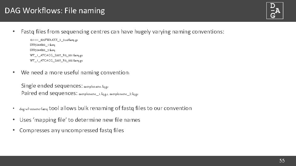
DAG Workflows: File naming • Fastq files from sequencing centres can have hugely varying naming conventions: 101111_620 FWAAXX_2_0. solfastq. gz SRR 5244800_1. fastq SRR 5244800_2. fastq WT_1_ATCACG_L 007_R 0_001. fastq. gz WT_1_ATCACG_L 007_R 0_002. fastq. gz • We need a more useful naming convention: Single ended sequences: samplename. fq. gz Paired end sequences: samplename_1. fq. gz, samplename_2. fq. gz • dag-wf-rename-fastq tool allows bulk renaming of fastq files to our convention • Uses ‘mapping file’ to determine new file names • Compresses any uncompressed fastq files 55

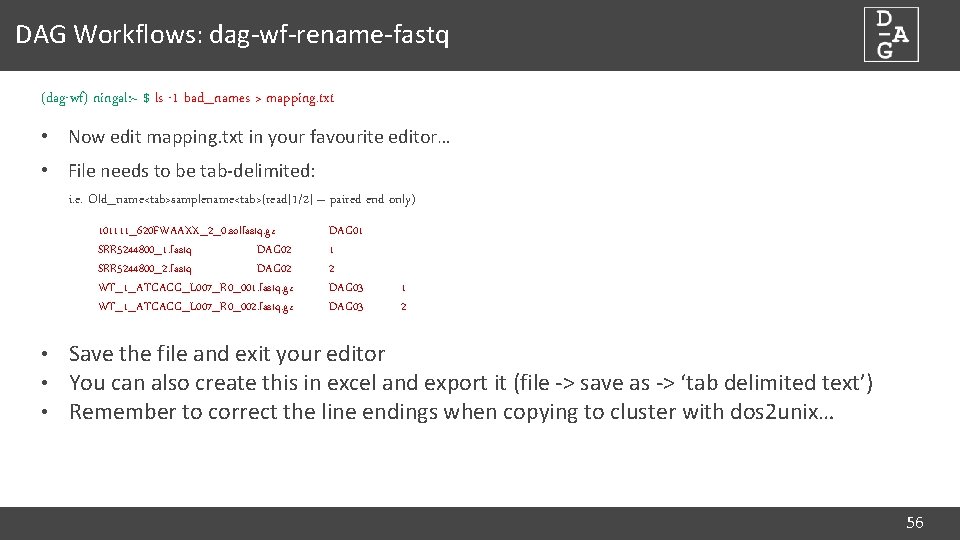
DAG Workflows: dag-wf-rename-fastq (dag-wf) ningal: ~ $ ls -1 bad_names > mapping. txt • Now edit mapping. txt in your favourite editor… • File needs to be tab-delimited: i. e. Old_name<tab>samplename<tab>(read[1/2] – paired end only) 101111_620 FWAAXX_2_0. solfastq. gz SRR 5244800_1. fastq DAG 02 SRR 5244800_2. fastq DAG 02 WT_1_ATCACG_L 007_R 0_001. fastq. gz WT_1_ATCACG_L 007_R 0_002. fastq. gz DAG 01 1 2 DAG 03 1 2 • Save the file and exit your editor • You can also create this in excel and export it (file -> save as -> ‘tab delimited text’) • Remember to correct the line endings when copying to cluster with dos 2 unix… 56

DAG Workflows: dag-wf-rename-fastq (dag-wf) ningal: ~ $ dag-wf-rename-fastq Usage: dag-wf-rename-files [-i inputdir] [-o outputdir] [-m mapping_file] [-h] Renames batches of files to make them amenable to running through DAG workflows Symbolic links are created in outputdir with a filename determined by the various fields in the mapping file. The required mapping file should be a tab delimited file containing the following fields: Original_filename Sample Read where: original_filename: the current name of the file sample: the sample name to which the file relates read: either '1' or '2' (not required for single-ended fastq files) Options: * -i: path to input directory containing files to rename * -o: path to output directory in which symlinks will be created * -m: mapping file of filename to sample mappings * -h: Display help • So give it a go…. 57

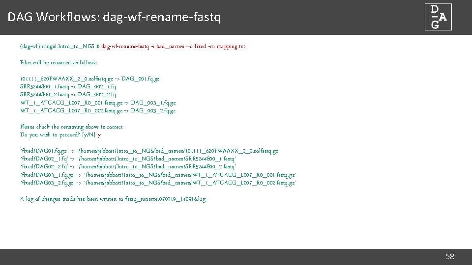
DAG Workflows: dag-wf-rename-fastq (dag-wf) ningal: Intro_to_NGS $ dag-wf-rename-fastq -i bad_names –o fixed -m mapping. txt Files will be renamed as follows: 101111_620 FWAAXX_2_0. solfastq. gz -> DAG_001. fq. gz SRR 5244800_1. fastq -> DAG_002_1. fq SRR 5244800_2. fastq -> DAG_002_2. fq WT_1_ATCACG_L 007_R 0_001. fastq. gz -> DAG_003_1. fq. gz WT_1_ATCACG_L 007_R 0_002. fastq. gz -> DAG_003_2. fq. gz Please check the renaming above is correct Do you wish to proceed? [y/N] y `fixed/DAG 01. fq. gz' -> `/homes/jabbott/Intro_to_NGS/bad_names/101111_620 FWAAXX_2_0. solfastq. gz' `fixed/DAG 02_1. fq' -> `/homes/jabbott/Intro_to_NGS/bad_names/SRR 5244800_1. fastq' `fixed/DAG 02_2. fq' -> `/homes/jabbott/Intro_to_NGS/bad_names/SRR 5244800_2. fastq' `fixed/DAG 03_1. fq. gz' -> `/homes/jabbott/Intro_to_NGS/bad_names/WT_1_ATCACG_L 007_R 0_001. fastq. gz' `fixed/DAG 03_2. fq. gz' -> `/homes/jabbott/Intro_to_NGS/bad_names/WT_1_ATCACG_L 007_R 0_002. fastq. gz' A log of changes made has been written to fastq_rename. 070319_140916. log 58

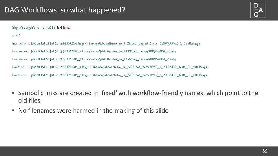
DAG Workflows: so what happened? (dag-wf) ningal: Intro_to_NGS $ ls -l fixed/ total 0 lrwxrwxrwx 1 jabbott lsd 75 Jul 31 13: 56 DAG 01. fq. gz -> /homes/jabbott/Intro_to_NGS/bad_names/101111_620 FWAAXX_2_0. solfastq. gz lrwxrwxrwx 1 jabbott lsd 61 Jul 31 13: 56 DAG 02_1. fq -> /homes/jabbott/Intro_to_NGS/bad_names/SRR 5244800_1. fastq lrwxrwxrwx 1 jabbott lsd 61 Jul 31 13: 56 DAG 02_2. fq -> /homes/jabbott/Intro_to_NGS/bad_names/SRR 5244800_2. fastq lrwxrwxrwx 1 jabbott lsd 75 Jul 31 13: 56 DAG 03_1. fq. gz -> /homes/jabbott/Intro_to_NGS/bad_names/WT_1_ATCACG_L 007_R 0_001. fastq. gz lrwxrwxrwx 1 jabbott lsd 75 Jul 31 13: 56 DAG 03_2. fq. gz -> /homes/jabbott/Intro_to_NGS/bad_names/WT_1_ATCACG_L 007_R 0_002. fastq. gz • Symbolic links are created in 'fixed' with workflow-friendly names, which point to the old files • No filenames were harmed in the making of this slide 59

DAG Workflows: workflow setup (dag-wf) ningal: ~ $ dag-wf-setup Usage: dag-wf-setup [-n name] [-d directory] [-w workflow] [-i inputdir] Options: * -n: Name of workflow job * -d: Directory to create for containing workflow files * -w: Workflow to initiate * -i: Directory containing input files for workflow * -c: Copy input files into workflow (default: use symlink) Available workflows: qc-pe, qc-se 60

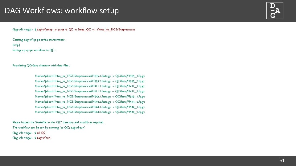
DAG Workflows: workflow setup (dag-wf) ningal: ~ $ dag-wf-setup -w qc-pe -d QC -n Strep_QC –i ~/Intro_to_NGS/Streptococcus Creating dag-wf-qc-pe conda environment [snip] Setting up qc-pe workflow in QC. . . Populating QC/fastq directory with data files. . . /homes/jabbott/Intro_to_NGS/Streptococcus/H 395. 1. fastq. gz -> QC/fastq/H 395_1. fq. gz /homes/jabbott/Intro_to_NGS/Streptococcus/H 395. 2. fastq. gz -> QC/fastq/H 395_2. fq. gz /homes/jabbott/Intro_to_NGS/Streptococcus/H 411. 1. fastq. gz -> QC/fastq/H 411_1. fq. gz /homes/jabbott/Intro_to_NGS/Streptococcus/H 411. 2. fastq. gz -> QC/fastq/H 411_2. fq. gz /homes/jabbott/Intro_to_NGS/Streptococcus/H 543. 1. fastq. gz -> QC/fastq/H 543_1. fq. gz /homes/jabbott/Intro_to_NGS/Streptococcus/H 543. 2. fastq. gz -> QC/fastq/H 543_2. fq. gz /homes/jabbott/Intro_to_NGS/Streptococcus/H 544. 1. fastq. gz -> QC/fastq/H 544_1. fq. gz /homes/jabbott/Intro_to_NGS/Streptococcus/H 544. 2. fastq. gz -> QC/fastq/H 544_2. fq. gz Please inspect the Snakefile in the 'QC' directory and modify as required. The workflow can be run by running 'cd QC; dag-wf-run' (dag-wf) ningal: ~ $ cd QC (dag-wf) ningal: ~ $ dag-wf-run 61

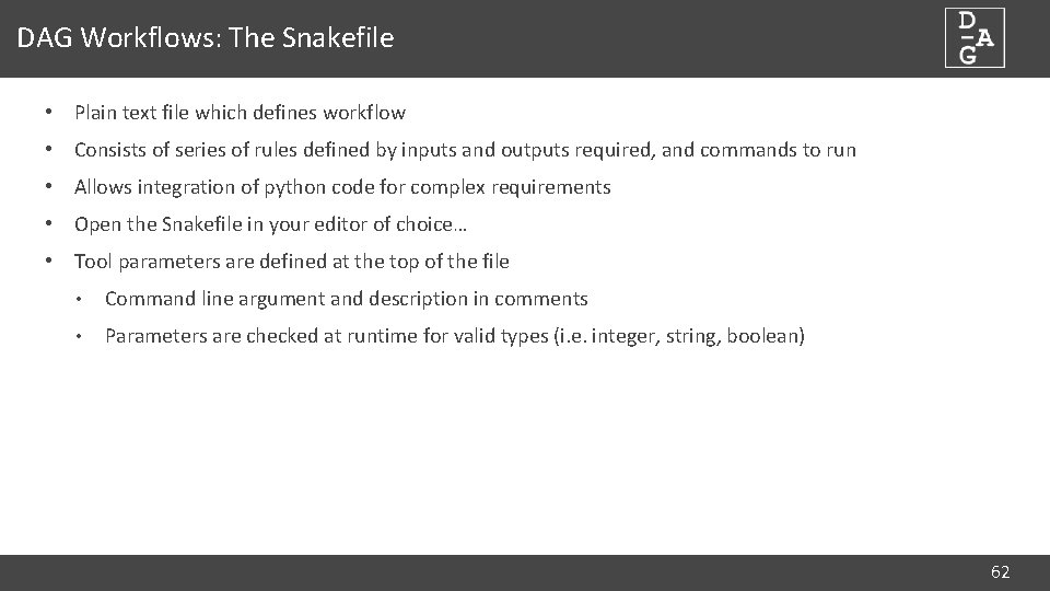
DAG Workflows: The Snakefile • Plain text file which defines workflow • Consists of series of rules defined by inputs and outputs required, and commands to run • Allows integration of python code for complex requirements • Open the Snakefile in your editor of choice… • Tool parameters are defined at the top of the file • Command line argument and description in comments • Parameters are checked at runtime for valid types (i. e. integer, string, boolean) 62

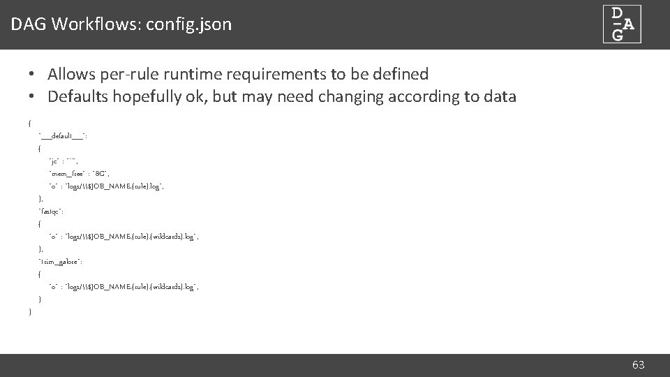
DAG Workflows: config. json • Allows per-rule runtime requirements to be defined • Defaults hopefully ok, but may need changing according to data { } "__default__": { "jc" : "''", "mem_free" : "8 G", "o" : "logs/\$JOB_NAME. {rule}. log", }, "fastqc": { "o" : "logs/\$JOB_NAME. {rule}. {wildcards}. log", }, "trim_galore": { "o" : "logs/\$JOB_NAME. {rule}. {wildcards}. log", } 63

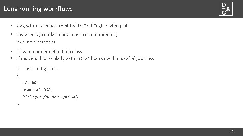
Long running workflows • dag-wf-run can be submitted to Grid Engine with qsub • Installed by conda so not in our current directory qsub $(which dag-wf-run) • Jobs run under default job class • If individual tasks likely to take > 24 hours need to use 'inf' job class • Edit config. json…. { "jc" : "inf", "mem_free" : "8 G", "o" : "logs/\$JOB_NAME. {rule}. log", }, 64

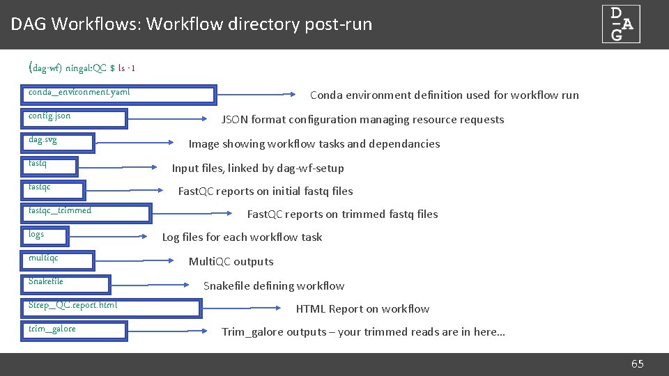
DAG Workflows: Workflow directory post-run (dag-wf) ningal: QC $ ls -1 conda_environment. yaml config. json dag. svg fastqc_trimmed logs multiqc Snakefile Strep_QC. report. html trim_galore Conda environment definition used for workflow run JSON format configuration managing resource requests Image showing workflow tasks and dependancies Input files, linked by dag-wf-setup Fast. QC reports on initial fastq files Fast. QC reports on trimmed fastq files Log files for each workflow task Multi. QC outputs Snakefile defining workflow HTML Report on workflow Trim_galore outputs – your trimmed reads are in here… 65

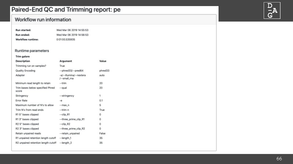
66

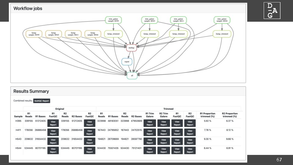
67

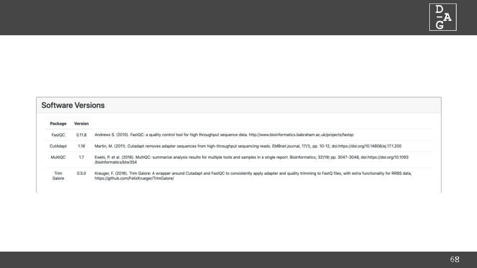
68

The Sequence Read Archive dundee. ac. uk http: //dag. compbio. dundee. ac. uk cb-dag@dundee. ac. uk @Uo. D_DAG Page

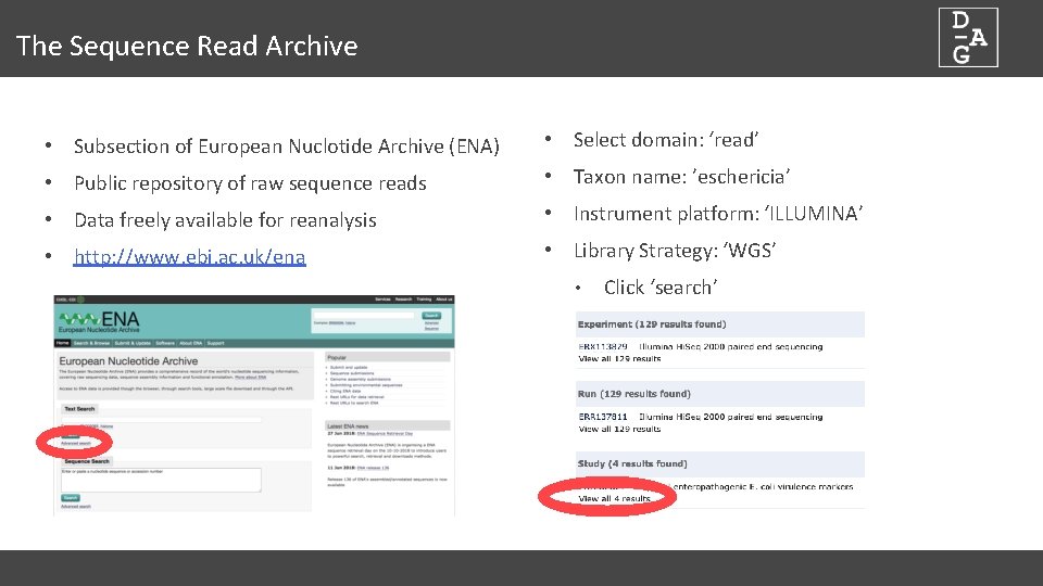
The Sequence Read Archive • Subsection of European Nuclotide Archive (ENA) • Select domain: ‘read’ • Public repository of raw sequence reads • Taxon name: ’eschericia’ • Data freely available for reanalysis • Instrument platform: ‘ILLUMINA’ • http: //www. ebi. ac. uk/ena • Library Strategy: ‘WGS’ • Click ‘search’

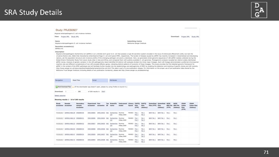
SRA Study Details 71

Summary We have covered: • Different approaches to sequencing • Library types (Single end/Paired end/Mate pair) • Sequence base quality • Sequence file formats • Sequence quality assessment • Remedial work for problematic sequences • Read trimming • Subsampling • Duplicate removal • Using DAG workflows for sequence QC • Finding publicly accessible sequence data from the SRA 72

Any Questions? http: //dag. compbio. dundee. ac. uk cb-dag@dundee. ac. uk @Uo. D_DAG 7