MODULE 13 DATA HANDLING n Collect organize and

MODULE - 13 DATA HANDLING

n Collect, organize and interpret univariate numerical data in order to determine: measures of central tendency (mean, median, mode) of grouped and ungrouped data, and know which is the most appropriate under given conditions; measures of dispersion: range, percentiles, quartiles, interquartiles, and semiinterquartile range.

Represent data effectively, choosing appropriately from: bar and compound bar graphs, histograms (grouped data) frequency charts , pie charts, line and broken line graphs n (L 04 AS 1) n

n When information is collected on a particular subject, the information collected is called data. n Many issues in the real world can be researched by collecting data and representing the data graphically in the form of bar graphs, pie charts, broken line graphs, histograms and frequency polygons.

Data handling involves the following: Collecting data n Sorting the data n Representing the data graphically n Interpreting results n Making conclusions n

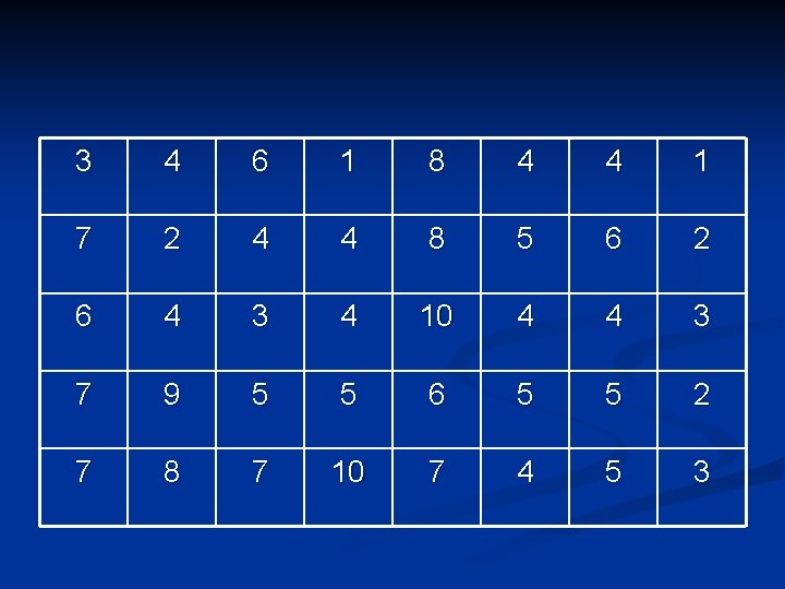
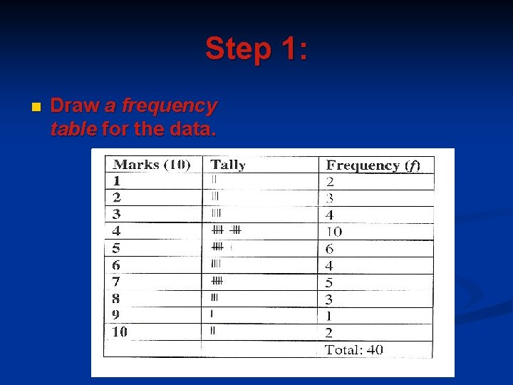
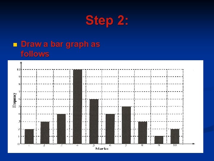
A. REPRESENTING UNGROUPED DATA GRAPHICALLY Bar Graphs n A bar graph is a diagram consisting of horizontal or vertical bars. n Example involving vertical bars: n A teacher has recorded the test marks of forty grade 10 learners in the table below. The test was out of 10 and she wants to represent the data graphically by using a bar graph. n

3 4 6 1 8 4 4 1 7 2 4 4 8 5 6 2 6 4 3 4 10 4 4 3 7 9 5 5 6 5 5 2 7 8 7 10 7 4 5 3

Step 1: n Draw a frequency table for the data.

Step 2: n Draw a bar graph as follows

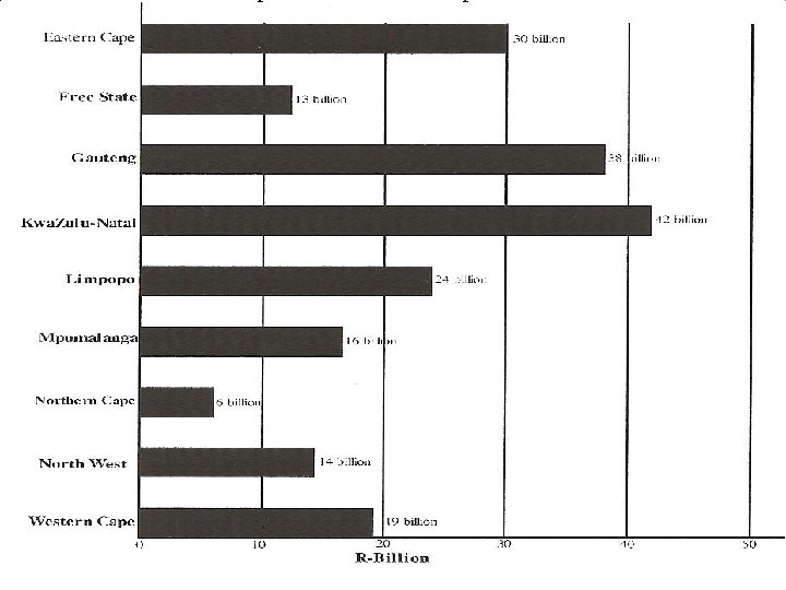
Example involving horizontal bars n In his Budget 2007 speech, Trevor Manuel allocated the following amounts in billions to the different provinces for Transport and communication:

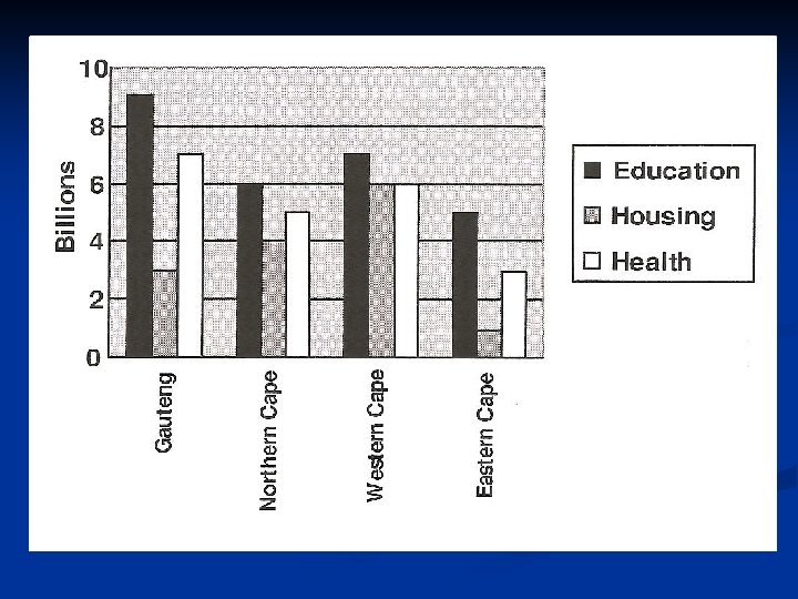
Example involving compound bar graphs n n These bar graphs are used when different sets of information are given on connected topics For example: In his Budget speech, Trevor Manuel allocated funds for Education, Housing and Health to the different provinces. The compound bar graph below represents the allocation of these three categories to four different provinces.

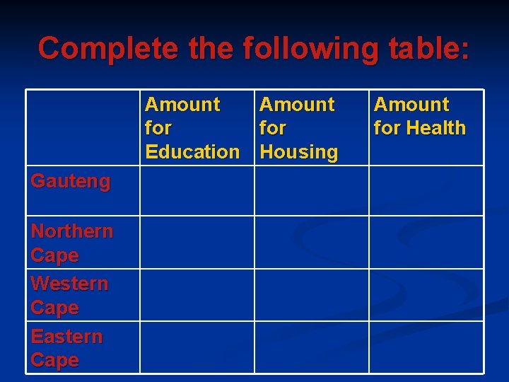
Complete the following table: Amount for Education Housing Gauteng Northern Cape Western Cape Eastern Cape Amount for Health

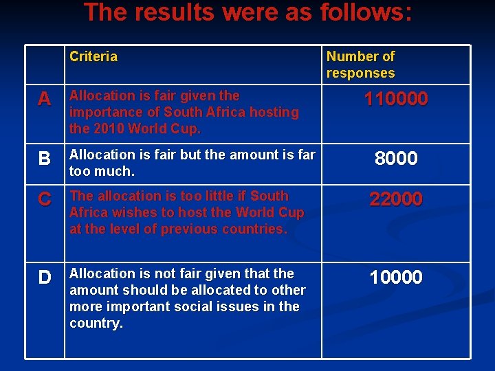
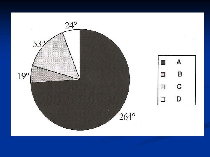
Pie Graphs n n n Pie graphs are circular in shape. The percentages per sector can be represented as degrees. The following example illustrates how to represent data on a pie graph. In a recent survey, a sample of 150 000 South Africans were asked to comment on Trevor Manual's allocation of 17, 4 billion rand to the 2010 Fifa World Cup.

The results were as follows: Criteria Number of responses A Allocation is fair given the importance of South Africa hosting the 2010 World Cup. B Allocation is fair but the amount is far too much. C The allocation is too little if South Africa wishes to host the World Cup at the level of previous countries. 22000 D Allocation is not fair given that the amount should be allocated to other more important social issues in the country. 10000 110000 8000

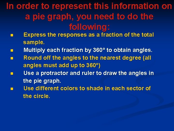
In order to represent this information on a pie graph, you need to do the following: n n n Express the responses as a fraction of the total sample. Multiply each fraction by 360° to obtain angles. Round off the angles to the nearest degree (all angles must add up to 360°) Use a protractor and ruler to draw the angles in the pie graph. Use different colors to shade in each sector of the circle.

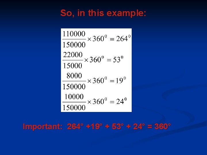
So, in this example: Important: 264° +19° + 53° + 24° = 360°

Broken line graphs represent information collected at different points. They do not contain information about situations in between these points.

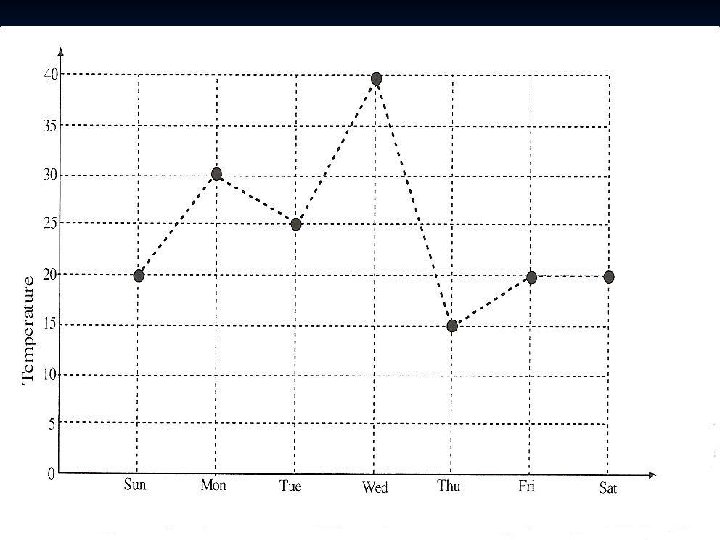
Example n The following graph represents the temperatures recorded at 13 h 00 each day from a particular Sunday to the following Saturday.

n n n n The temperature on Sunday was 20°C and on Monday it was 30°C. The temperature at any other time between 13 h 00 on Sunday and 13 h 00 on Monday cannot be read off from the graph, because we were only given the temperatures at 13 h 00 each day. The temperature might have increased or decreased between 13 h 00 on Sunday and 13 h 00 on Monday. That is why the line is dotted (broken) between the 13 h 00 points. Notice that the highest temperature at 13 h 00 was on Wednesday. Whether or not the temperature was higher than this between the 13 h 00 points cannot be known from the graph. We can try to use the graph to predict when the temperatures will be the highest. In this case, it seems that the temperatures are highest during the middle of the week.

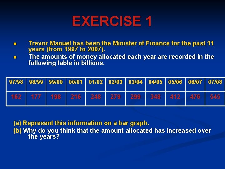
EXERCISE 1 n n Trevor Manuel has been the Minister of Finance for the past 11 years (from 1997 to 2007). The amounts of money allocated each year are recorded in the following table in billions. 97/98 98/99 99/00 00/01 01/02 02/03 03/04 04/05 05/06 06/07 07/08 162 177 198 216 248 279 299 348 412 476 545 (a) Represent this information on a bar graph. (b) Why do you think that the amount allocated has increased over the years?

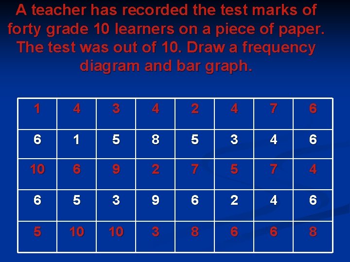
A teacher has recorded the test marks of forty grade 10 learners on a piece of paper. The test was out of 10. Draw a frequency diagram and bar graph. 1 4 3 4 2 4 7 6 6 1 5 8 5 3 4 6 10 6 9 2 7 5 7 4 6 5 3 9 6 2 4 6 5 10 10 3 8 6 6 8

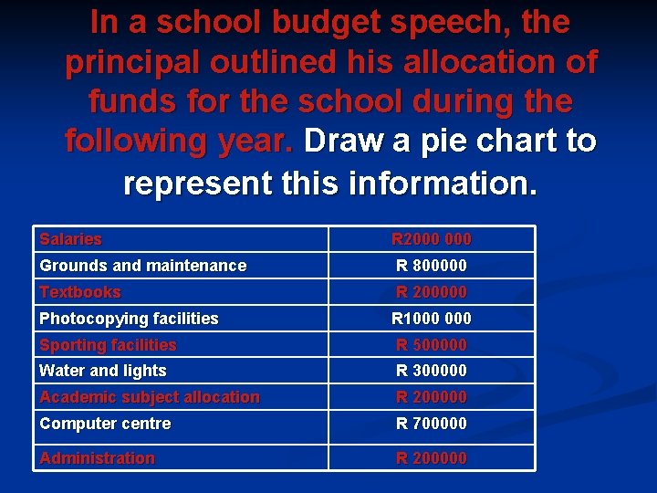
In a school budget speech, the principal outlined his allocation of funds for the school during the following year. Draw a pie chart to represent this information. Salaries R 2000 Grounds and maintenance R 800000 Textbooks R 200000 Photocopying facilities R 1000 Sporting facilities R 500000 Water and lights R 300000 Academic subject allocation R 200000 Computer centre R 700000 Administration R 200000

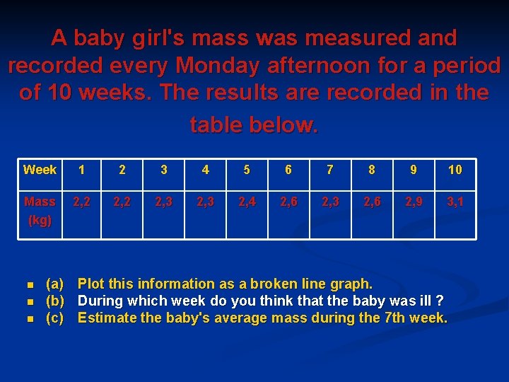
A baby girl's mass was measured and recorded every Monday afternoon for a period of 10 weeks. The results are recorded in the table below. Week 1 2 3 4 5 6 7 8 9 10 Mass (kg) 2, 2 2, 3 2, 4 2, 6 2, 3 2, 6 2, 9 3, 1 n n n (a) Plot this information as a broken line graph. (b) During which week do you think that the baby was ill ? (c) Estimate the baby's average mass during the 7 th week.

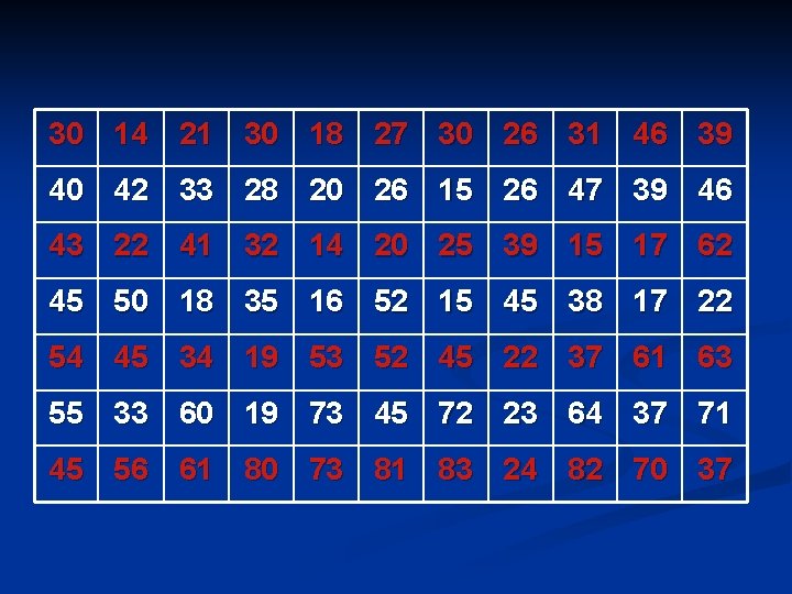
REPRESENTING GROUPED DATA GRAPHICALLY n n n It often happens that the data you are dealing with is too large making it necessary to group the data into what are called class intervals. The information can be represented by means of stem and leaf diagrams, histograms and frequency polygons. Example A health and fitness group conducted a survey in the area to find out which age group most frequently makes use of gyms. The group determined the ages of their current clients. Gym contracts were then marketed to this age group in the area. The ages of current clients were recorded and then sorted.

30 14 21 30 18 27 30 26 31 46 39 40 42 33 28 20 26 15 26 47 39 46 43 22 41 32 14 20 25 39 15 17 62 45 50 18 35 16 52 15 45 38 17 22 54 45 34 19 53 52 45 22 37 61 63 55 33 60 19 73 45 72 23 64 37 71 45 56 61 80 73 81 83 24 82 70 37

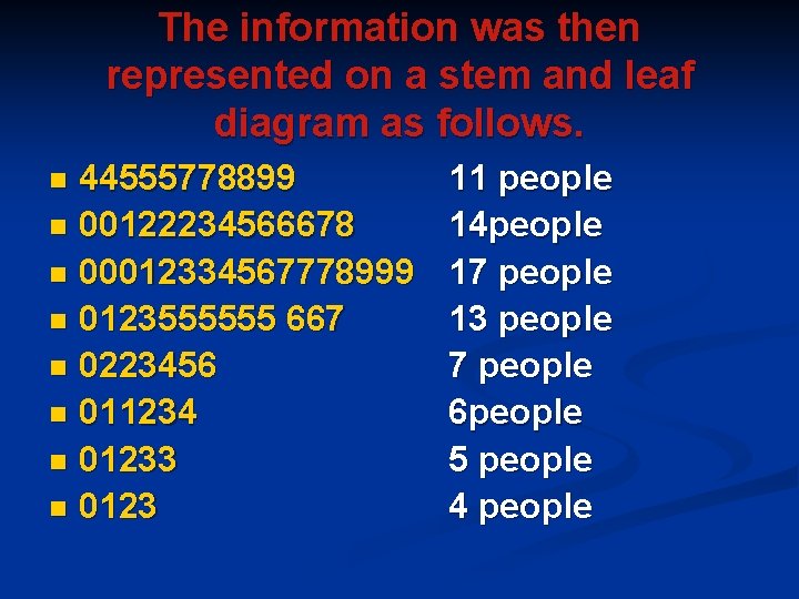
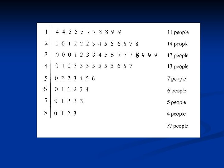
The information was then represented on a stem and leaf diagram as follows. 44555778899 n 00122234566678 n 00012334567778999 n 0123555555 667 n 0223456 n 011234 n 01233 n 0123 n 11 people 14 people 17 people 13 people 7 people 6 people 5 people 4 people

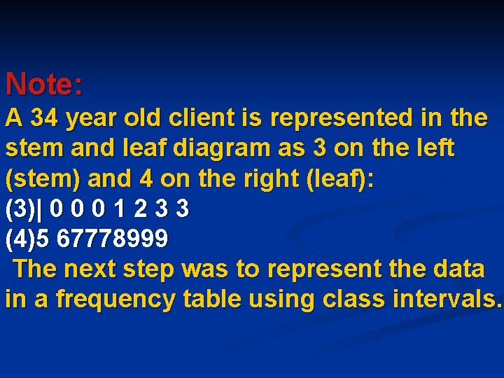
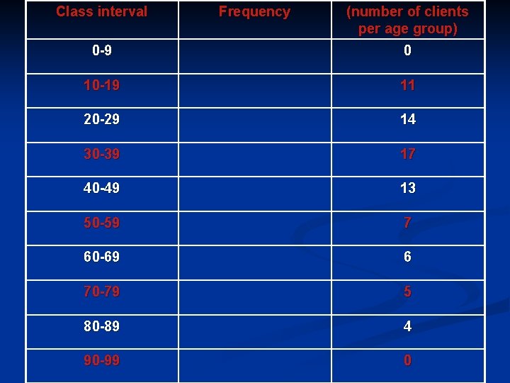
Note: A 34 year old client is represented in the stem and leaf diagram as 3 on the left (stem) and 4 on the right (leaf): (3)| 0 0 0 1 2 3 3 (4)5 67778999 The next step was to represent the data in a frequency table using class intervals.

Class interval Frequency (number of clients per age group) 0 -9 0 10 -19 11 20 -29 14 30 -39 17 40 -49 13 50 -59 7 60 -69 6 70 -79 5 80 -89 4 90 -99 0

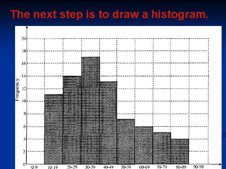
The next step is to draw a histogram.

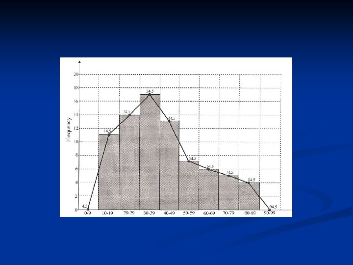
n n n Notice: In a histogram, there are no gaps between the bars. The data is continuous from 10 to 89 years. Each bar represents a class interval and the frequency is read off from the vertical axis (height of each bar). The next step is to draw a frequency polygon onto the histogram. A frequency polygon is similar to a line graph. The difference here is that with a frequency polygon, the class midpoints of each histogram are joined. Pretend there is an imaginary histogram to the left of the first histogram and to the right of the last histogram. Find the midpoints of these imaginary class intervals. Join all points to form a polygon.

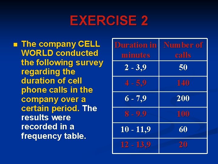
EXERCISE 2 n The company CELL WORLD conducted the following survey regarding the duration of cell phone calls in the company over a certain period. The results were recorded in a frequency table. Duration in Number of minutes calls 2 - 3, 9 50 4 - 5, 9 140 6 - 7, 9 200 8 - 9. 9 100 10 - 11, 9 60 12 - 13, 9 20

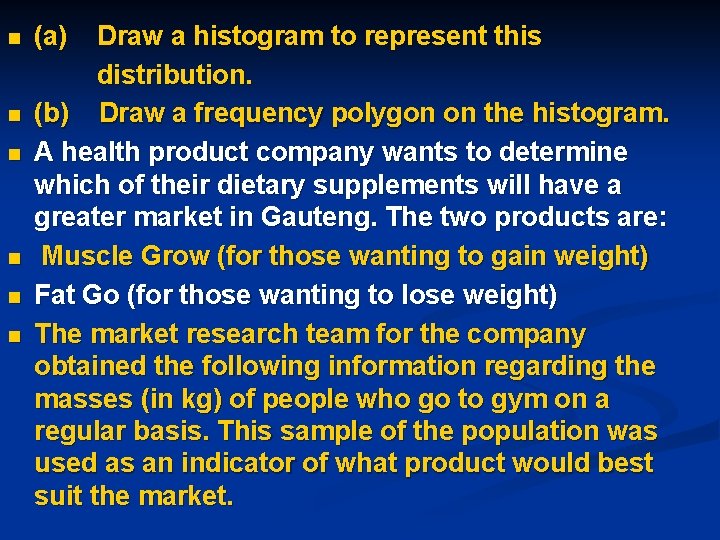
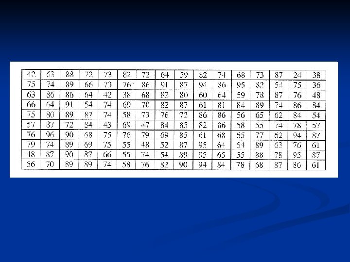
n n n (a) Draw a histogram to represent this distribution. (b) Draw a frequency polygon on the histogram. A health product company wants to determine which of their dietary supplements will have a greater market in Gauteng. The two products are: Muscle Grow (for those wanting to gain weight) Fat Go (for those wanting to lose weight) The market research team for the company obtained the following information regarding the masses (in kg) of people who go to gym on a regular basis. This sample of the population was used as an indicator of what product would best suit the market.

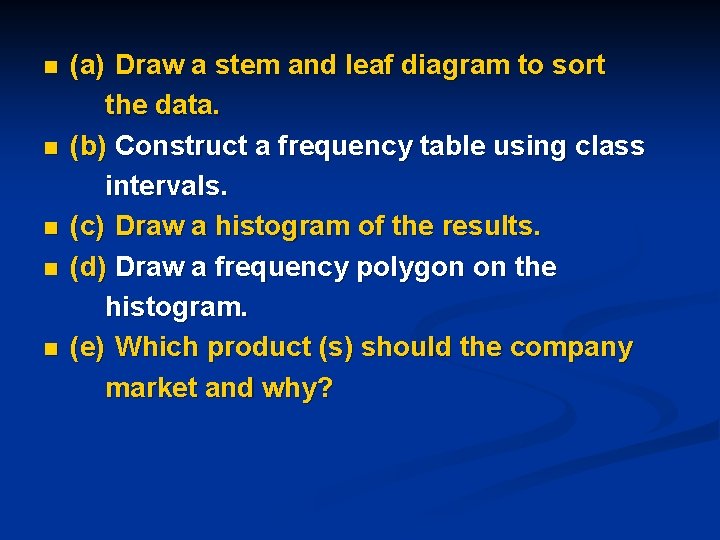
n n n (a) Draw a stem and leaf diagram to sort the data. (b) Construct a frequency table using class intervals. (c) Draw a histogram of the results. (d) Draw a frequency polygon on the histogram. (e) Which product (s) should the company market and why?

MEASURES OF CENTRAL TENDENCY (UNGROUPED DATA) n n n One set of data can be compared with another set of data by using measures of central tendency: the mean, median and mode. The Mean This measure of central tendency is the most commonly used of all three. Teachers work out the class average for a test and this average is called the mean. You obtain the mean by adding up all scores and then dividing by the total number of scores. The mean can be distorted if you have a small class and one or two learners do badly on the test. The average will be lower than if you have a larger class. This also works the other if one or more learners do very well. The average will tend to be too high as compared with a larger class.

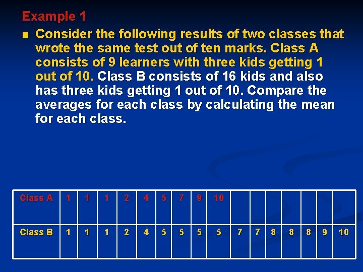
Example 1 n Consider the following results of two classes that wrote the same test out of ten marks. Class A consists of 9 learners with three kids getting 1 out of 10. Class B consists of 16 kids and also has three kids getting 1 out of 10. Compare the averages for each class by calculating the mean for each class. Class A 1 1 1 2 4 5 7 9 10 Class B 1 1 1 2 4 5 5 7 7 8 8 8 9 10

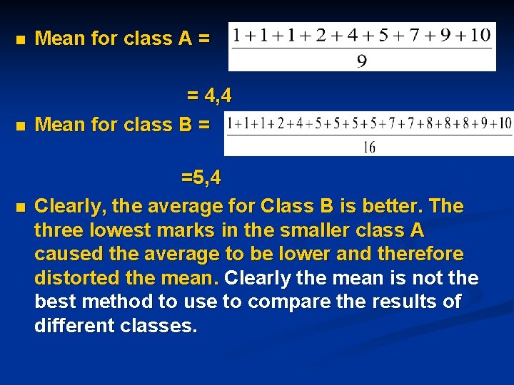
n Mean for class A = n = 4, 4 Mean for class B = n =5, 4 Clearly, the average for Class B is better. The three lowest marks in the smaller class A caused the average to be lower and therefore distorted the mean. Clearly the mean is not the best method to use to compare the results of different classes.

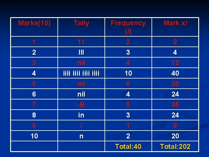
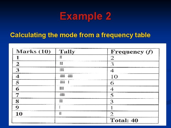
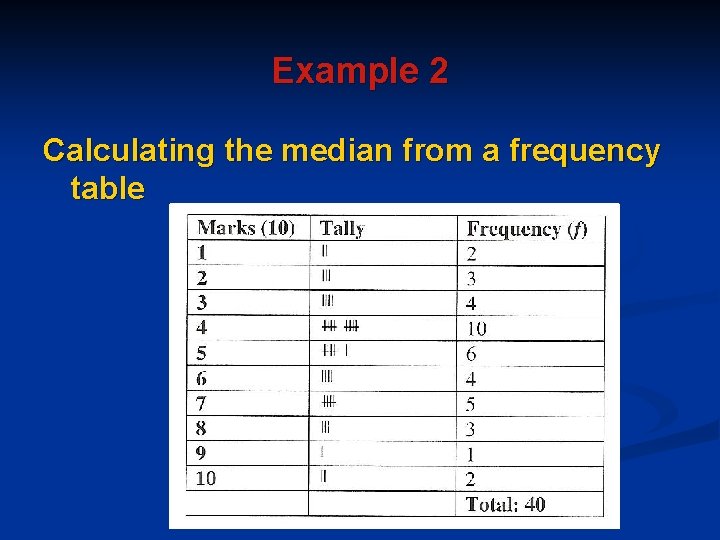
Example 2 (Calculating the mean from a frequency table) n Consider the example of the teacher who recorded the test marks of forty grade 10 learners. The data was represented in a frequency table. To calculate the mean, first multiply each mark by its frequency (fourth column). Then add up all entries in the fourth column. Now divide the sum of all marks (total in fourth column) by the total number of marks (third column).

Marks(10) Tally 1 2 11 III 3 4 5 6 7 8 9 10 nil iiii mi nil -B in i n Frequency (/) 2 3 4 10 6 4 5 3 1 2 Total: 40 Mark x/ 2 4 12 40 30 24 35 24 9 20 Total: 202

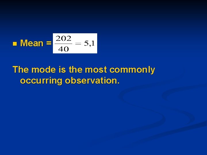
n Mean = The mode is the most commonly occurring observation.

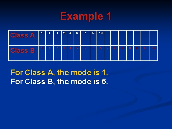
Example 1 Class A 1 1 1 2 4 5 7 9 10 Class B 1 1 1 2 4 5 5 7 For Class A, the mode is 1. For Class B, the mode is 5. 7 8 8 8 9 10

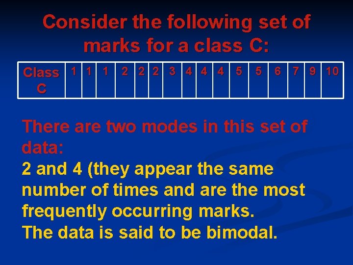
Consider the following set of marks for a class C: Class 1 1 1 2 2 2 3 4 4 4 5 5 6 7 9 10 C There are two modes in this set of data: 2 and 4 (they appear the same number of times and are the most frequently occurring marks. The data is said to be bimodal.

Example 2 Calculating the mode from a frequency table

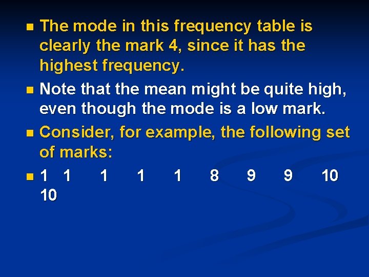
The mode in this frequency table is clearly the mark 4, since it has the highest frequency. n Note that the mean might be quite high, even though the mode is a low mark. n Consider, for example, the following set of marks: n 1 1 1 8 9 9 10 10 n

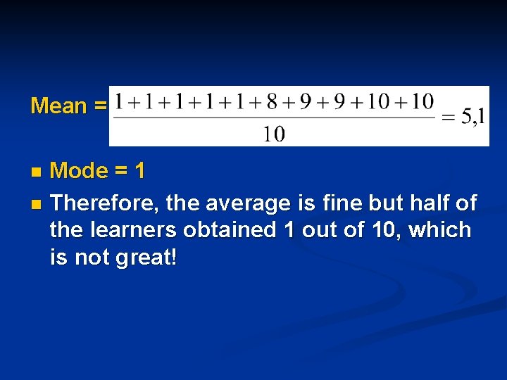
Mean = Mode = 1 n Therefore, the average is fine but half of the learners obtained 1 out of 10, which is not great! n

The Median n The median is the middlemost score (for an odd number of scores) and the average of the two middle scores (for an even number of scores). The scores should first be arranged in increasing order before the median can be calculated. The median is not affected by extremely high or low values and is therefore a good measure of central tendency.

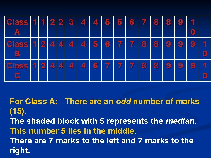
Example 1 Consider the following set of marks for a class test (out of 10) for three classes.

Class A Class B Class C 1 1 2 2 3 4 4 5 5 6 7 8 8 9 1 0 1 2 4 4 5 6 7 7 8 8 9 9 9 1 0 1 2 4 4 6 7 7 7 8 8 9 9 9 1 0 For Class A: There an odd number of marks (15). The shaded block with 5 represents the median. This number 5 lies in the middle. There are 7 marks to the left and 7 marks to the right.

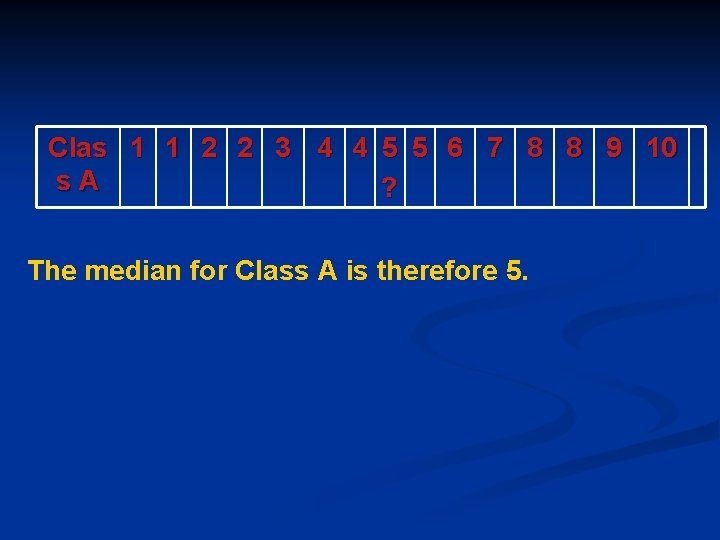
Clas 1 1 2 2 3 4 4 5 5 6 7 8 8 9 10 s. A ? The median for Class A is therefore 5.

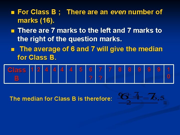
n n n For Class B ; There an even number of marks (16). There are 7 marks to the left and 7 marks to the right of the question marks. The average of 6 and 7 will give the median for Class B. Class 1 2 4 4 5 6 7 7 8 8 9 9 9 1 0 ? ? B The median for Class B is therefore:

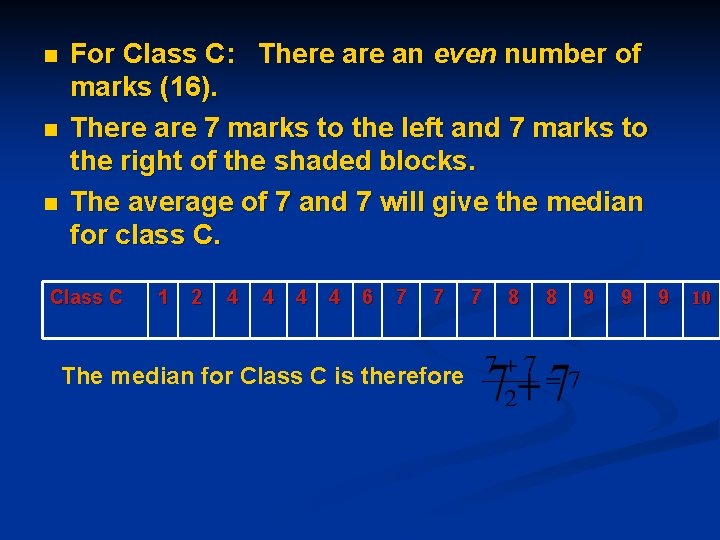
n n n For Class C: There an even number of marks (16). There are 7 marks to the left and 7 marks to the right of the shaded blocks. The average of 7 and 7 will give the median for class C. Class C 1 2 4 4 6 7 7 The median for Class C is therefore 7 8 8 9 9 9 10

Example 2 Calculating the median from a frequency table

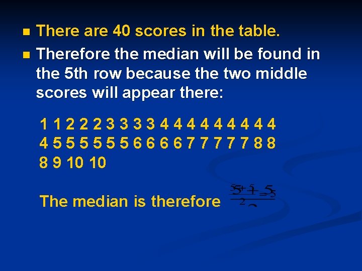
There are 40 scores in the table. n Therefore the median will be found in the 5 th row because the two middle scores will appear there: n 11222333344444 455555566667777788 8 9 10 10 The median is therefore

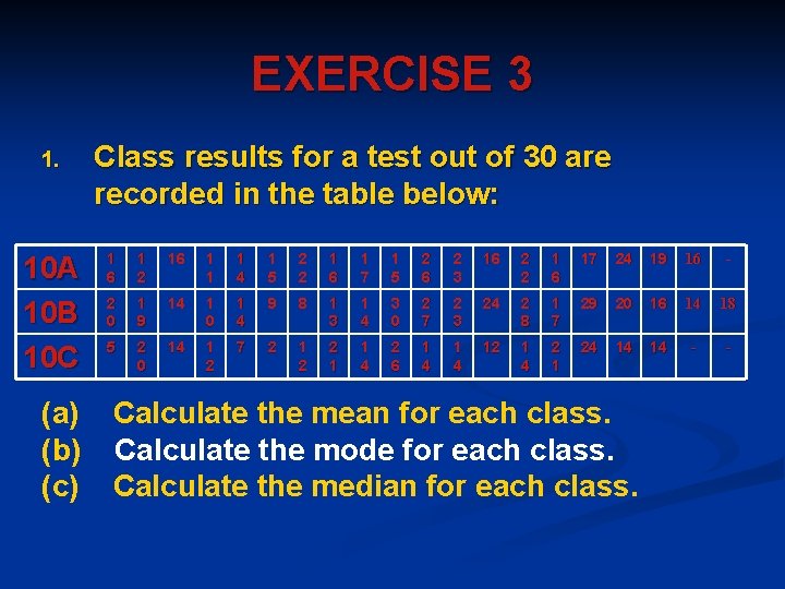
EXERCISE 3 1. 10 A 10 B 10 C (a) (b) (c) Class results for a test out of 30 are recorded in the table below: 1 6 1 2 16 1 1 1 4 1 5 2 2 1 6 1 7 1 5 2 6 2 3 16 2 2 1 6 17 24 19 16 - 2 0 1 9 14 1 0 1 4 9 8 1 3 1 4 3 0 2 7 2 3 24 2 8 1 7 29 20 16 14 18 5 2 0 14 1 2 7 2 1 2 2 1 1 4 2 6 1 4 12 1 4 2 1 24 14 14 - - Calculate the mean for each class. Calculate the mode for each class. Calculate the median for each class.

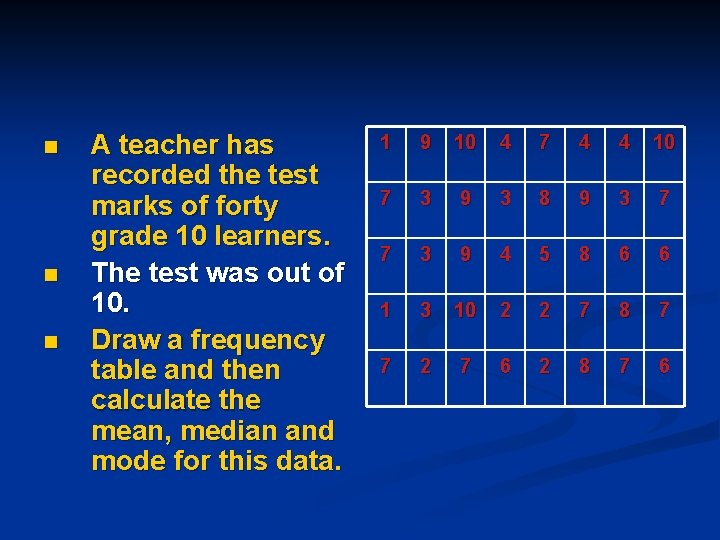
n n n A teacher has recorded the test marks of forty grade 10 learners. The test was out of 10. Draw a frequency table and then calculate the mean, median and mode for this data. 1 9 10 4 7 4 4 10 7 3 9 3 8 9 3 7 7 3 9 4 5 8 6 6 1 3 10 2 2 7 8 7 7 2 7 6 2 8 7 6

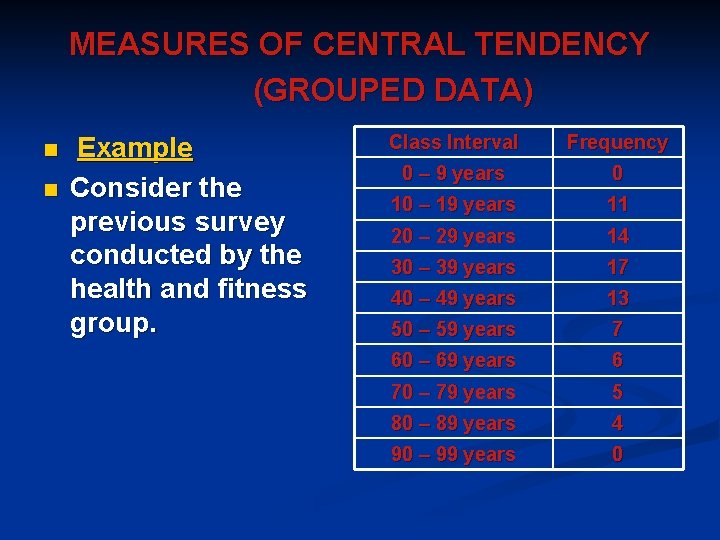
MEASURES OF CENTRAL TENDENCY (GROUPED DATA) n n Example Consider the previous survey conducted by the health and fitness group. Class Interval Frequency 0 – 9 years 0 10 – 19 years 11 20 – 29 years 14 30 – 39 years 17 40 – 49 years 13 50 – 59 years 7 60 – 69 years 6 70 – 79 years 5 80 – 89 years 4 90 – 99 years 0

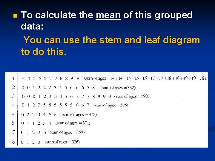
n To calculate the mean of this grouped data: You can use the stem and leaf diagram to do this.

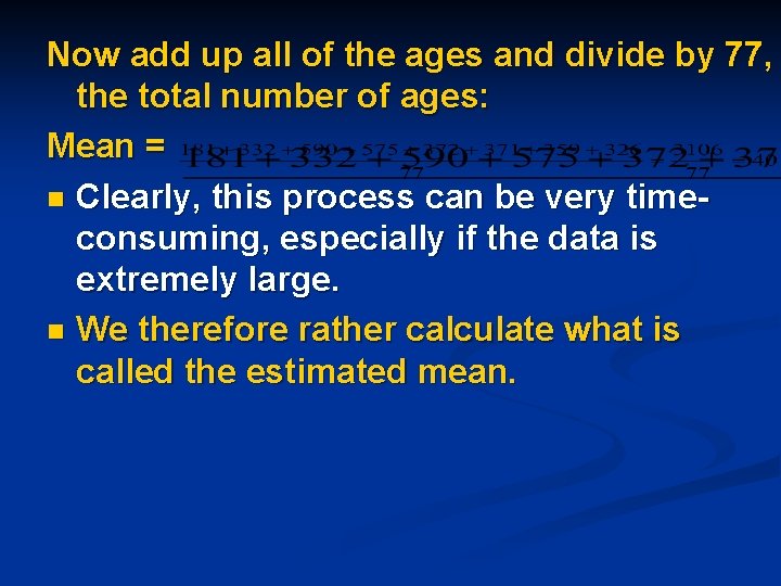
Now add up all of the ages and divide by 77, the total number of ages: Mean = n Clearly, this process can be very timeconsuming, especially if the data is extremely large. n We therefore rather calculate what is called the estimated mean.

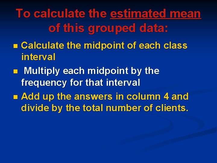
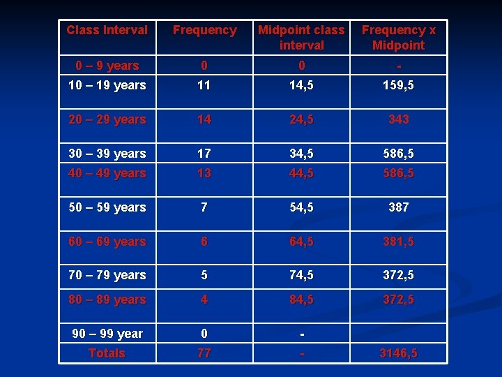
To calculate the estimated mean of this grouped data: Calculate the midpoint of each class interval n Multiply each midpoint by the frequency for that interval n Add up the answers in column 4 and divide by the total number of clients. n

Class Interval Frequency Midpoint class interval Frequency x Midpoint 0 – 9 years 0 0 - 10 – 19 years 11 14, 5 159, 5 20 – 29 years 14 24, 5 343 30 – 39 years 17 34, 5 586, 5 40 – 49 years 13 44, 5 586, 5 50 – 59 years 7 54, 5 387 60 – 69 years 6 64, 5 381, 5 70 – 79 years 5 74, 5 372, 5 80 – 89 years 4 84, 5 372, 5 90 – 99 year 0 - Totals 77 - 3146, 5

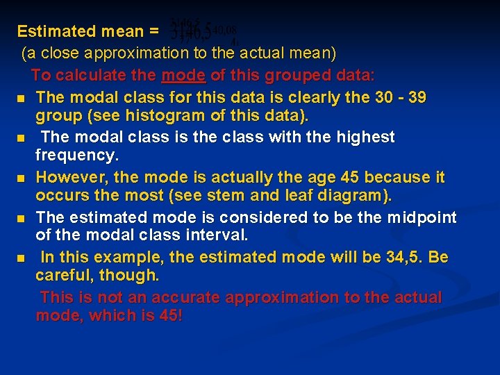
Estimated mean = (a close approximation to the actual mean) To calculate the mode of this grouped data: n The modal class for this data is clearly the 30 - 39 group (see histogram of this data). n The modal class is the class with the highest frequency. n However, the mode is actually the age 45 because it occurs the most (see stem and leaf diagram). n The estimated mode is considered to be the midpoint of the modal class interval. n In this example, the estimated mode will be 34, 5. Be careful, though. This is not an accurate approximation to the actual mode, which is 45!

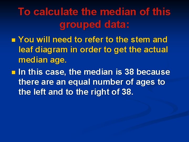
To calculate the median of this grouped data: You will need to refer to the stem and leaf diagram in order to get the actual median age. n In this case, the median is 38 because there an equal number of ages to the left and to the right of 38. n

EXERCISE 4 1. Refer to Exercise 2 Question 1. n (a) In which interval does the mode lie ? n (b) In which interval does the median lie ?

2. n n n Refer to Exercise 2 Question 2. For this data, calculate: (a) The estimated mean. (b) The mode. (c) The median.

E. MEASURES OF DISPERSION n n n n n Measures of dispersion help us to determine how data is spread around the mean or median. This enables one to establish whether the data is grouped closely or scattered more widely. The measures of dispersion dealt with in this module are: Range Quartiles Deciles Percentiles Interquartile range Semi-interquartile range

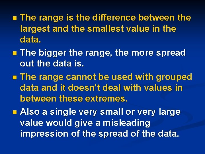
The range is the difference between the largest and the smallest value in the data. n The bigger the range, the more spread out the data is. n The range cannot be used with grouped data and it doesn't deal with values in between these extremes. n Also a single very small or very large value would give a misleading impression of the spread of the data. n

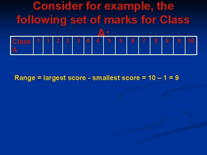
Consider for example, the following set of marks for Class A: 1 1 2 2 3 4 4 5 5 6 7 8 8 9 10 Class A Range = largest score - smallest score = 10 – 1 = 9

Quartiles are measures of dispersion around the median, which is a better measure of central tendency. n The median divides the data into two halves. n The quartiles further subdivide the data into quarters. n

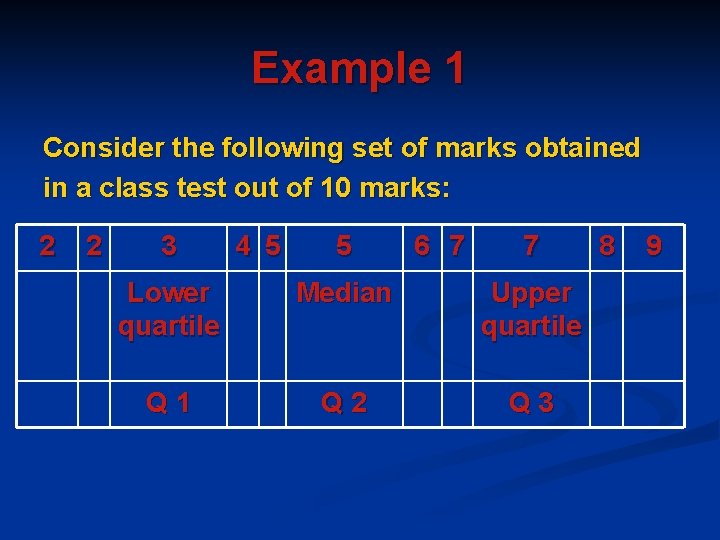
Example 1 Consider the following set of marks obtained in a class test out of 10 marks: 2 2 3 4 5 5 6 7 7 Lower quartile Median Upper quartile Q 1 Q 2 Q 3 8 9

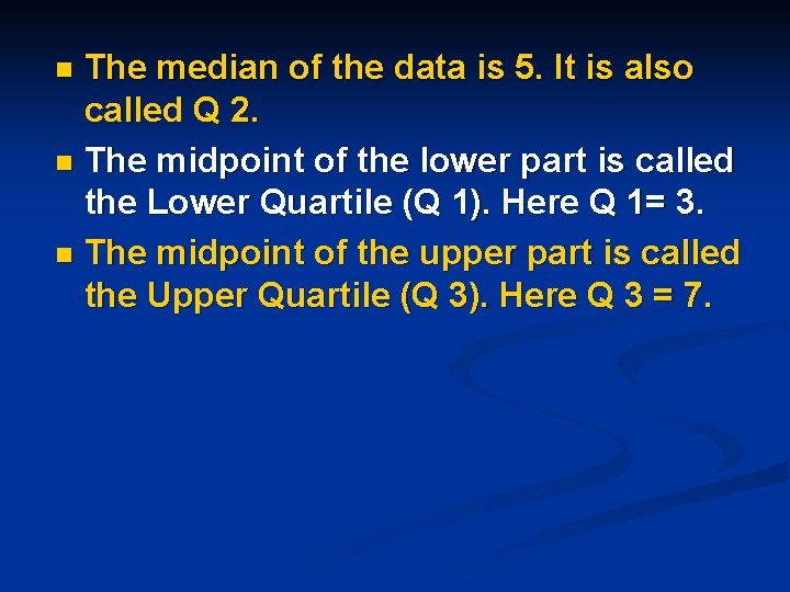
The median of the data is 5. It is also called Q 2. n The midpoint of the lower part is called the Lower Quartile (Q 1). Here Q 1= 3. n The midpoint of the upper part is called the Upper Quartile (Q 3). Here Q 3 = 7. n

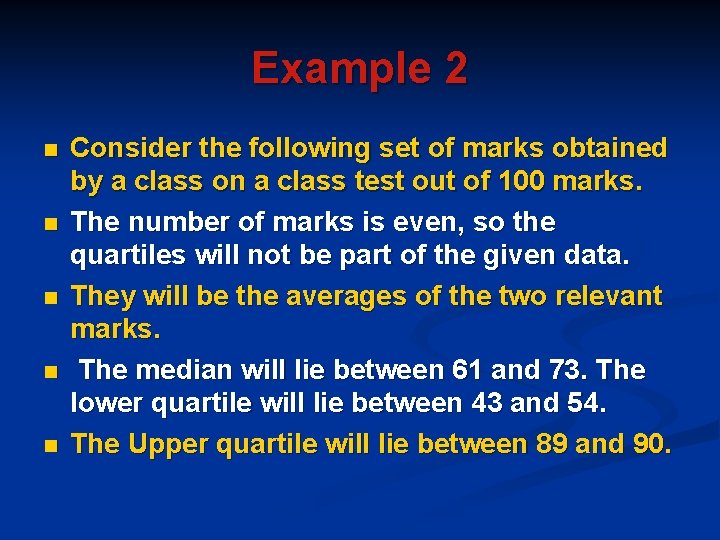
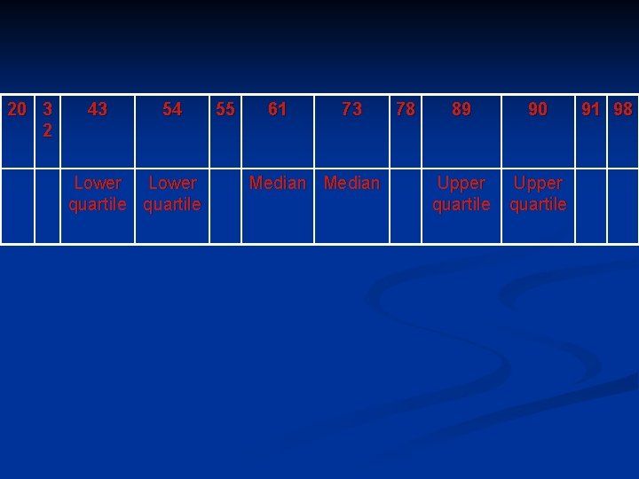
Example 2 n n n Consider the following set of marks obtained by a class on a class test out of 100 marks. The number of marks is even, so the quartiles will not be part of the given data. They will be the averages of the two relevant marks. The median will lie between 61 and 73. The lower quartile will lie between 43 and 54. The Upper quartile will lie between 89 and 90.

20 3 2 43 54 Lower quartile 55 61 73 Median 78 89 90 Upper quartile 91 98

Deciles and Percentiles Deciles subdivide the data into tenths. n Percentiles divide the data into hundredths n

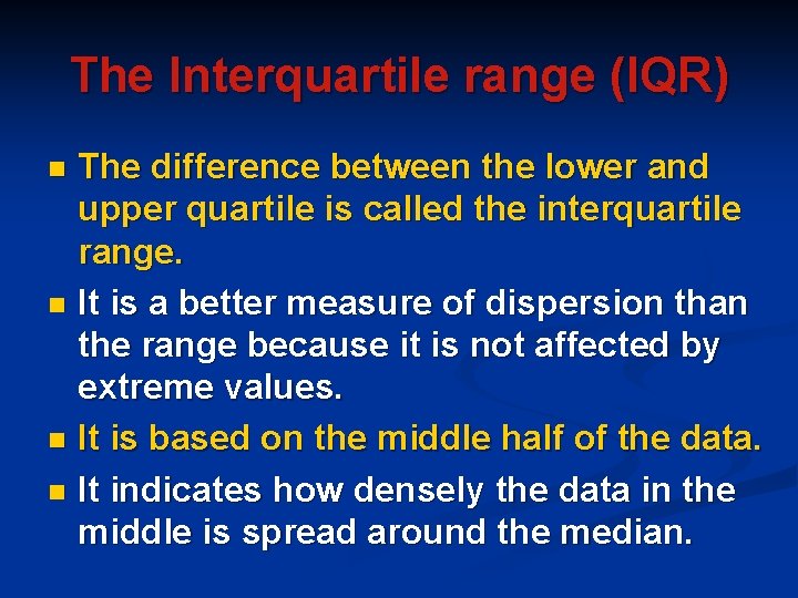
The Interquartile range (IQR) The difference between the lower and upper quartile is called the interquartile range. n It is a better measure of dispersion than the range because it is not affected by extreme values. n It is based on the middle half of the data. n It indicates how densely the data in the middle is spread around the median. n

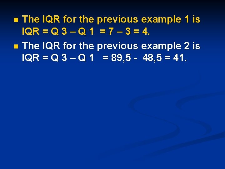
The IQR for the previous example 1 is IQR = Q 3 – Q 1 = 7 – 3 = 4. n The IQR for the previous example 2 is IQR = Q 3 – Q 1 = 89, 5 - 48, 5 = 41. n

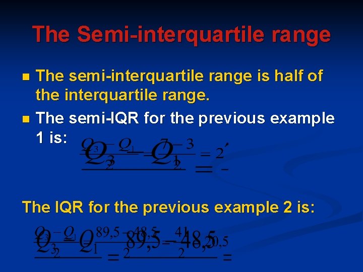
The Semi-interquartile range The semi-interquartile range is half of the interquartile range. n The semi-IQR for the previous example 1 is: n The IQR for the previous example 2 is:

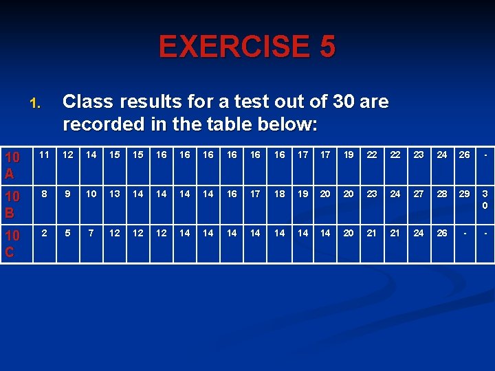
EXERCISE 5 Class results for a test out of 30 are recorded in the table below: 1. 10 A 11 12 14 15 15 16 16 16 17 17 19 22 22 23 24 26 - 10 B 8 9 10 13 14 14 16 17 18 19 20 20 23 24 27 28 29 3 0 10 C 2 5 7 12 12 12 14 14 20 21 21 24 26 - -

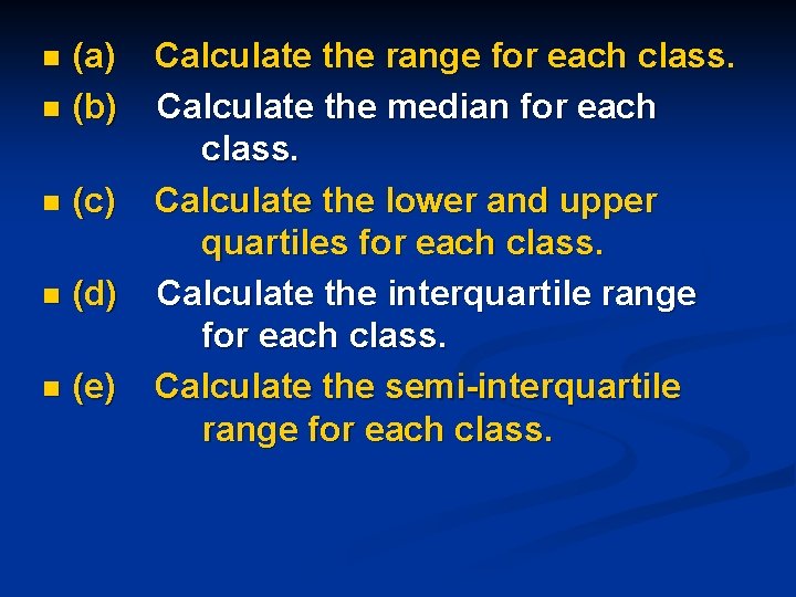
(a) n (b) n n (c) n (d) n (e) Calculate the range for each class. Calculate the median for each class. Calculate the lower and upper quartiles for each class. Calculate the interquartile range for each class. Calculate the semi-interquartile range for each class.

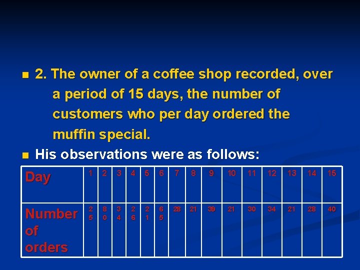
n n 2. The owner of a coffee shop recorded, over a period of 15 days, the number of customers who per day ordered the muffin special. His observations were as follows: Day 1 2 3 4 5 6 7 8 9 10 11 12 13 14 15 Number of orders 2 5 8 0 3 4 2 6 2 1 6 5 28 21 39 21 30 34 21 28 40

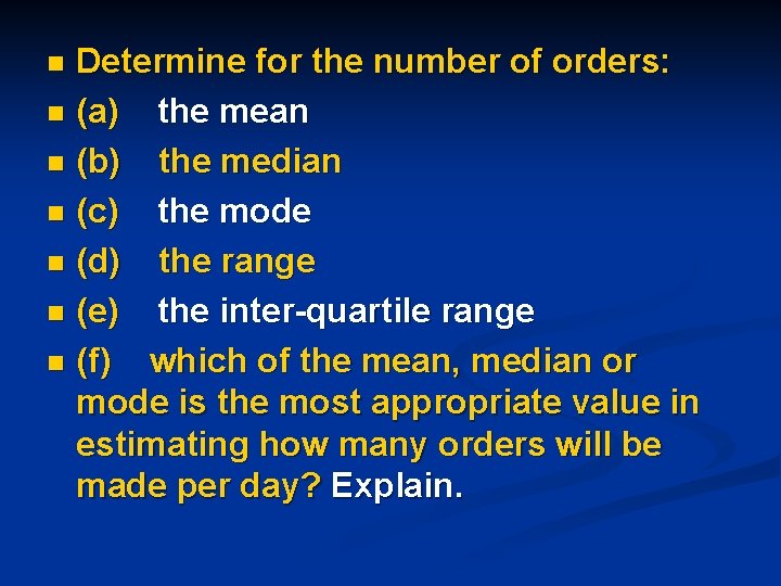
Determine for the number of orders: n (a) the mean n (b) the median n (c) the mode n (d) the range n (e) the inter-quartile range n (f) which of the mean, median or mode is the most appropriate value in estimating how many orders will be made per day? Explain. n

PROJECT ON DATA HANDLING n n n n You want to open your own business franchise in the area. Some of the franchises you are interested in exploring are the following: Restaurants Clothing stores Coffee shops/ Tea Gardens Computer stores You want to determine which franchise will be the most profitable for you. For example, if you want to open a restaurant, you will want to know which restaurant is the most popular for the area. Do you want to open a Nando’s or Ocean Basket?

PART 1 n n Choose a type of franchise you are interested in. Then design a questionnaire to find out which of the different names are the most popular. Draw up a tally sheet and then spend a few weekends at shopping malls in the area recording what people's favorite places are. Make sure that you interview a large sample of people.

PART 2 Now represent the data you have collected in a frequency diagram and then graphically (bar graph and pie chart). n You can do this quite effectively using a computer. n

PART 3 n n n Now start to analyze your results using the graphs. State which measure of central tendency will be the most appropriate for your data. Make conclusions as to what franchise you are going to open. Discuss factors that might adversely affect the business and factors that will help the business to succeed and be profitable. At the end of this task, you must present PART 1, 2 and 3 in a project format. Each part will be allocated a mark.

You will be assessed on the amount of effort put in as well as whether your findings are valid - will the business work! Enjoy!