DETERMINATION OF MOLECULAR WEIGHT OF POLYMERS Introduction Molecular


-Sv. • Known concentration of solution is taken solution Solvent • x₁")
 Low molecular weight High molecular weight Direction of the centrifugal force X")
-Mw • 15000 rev/min • S=D (Rate of Sedimentation is equal to")


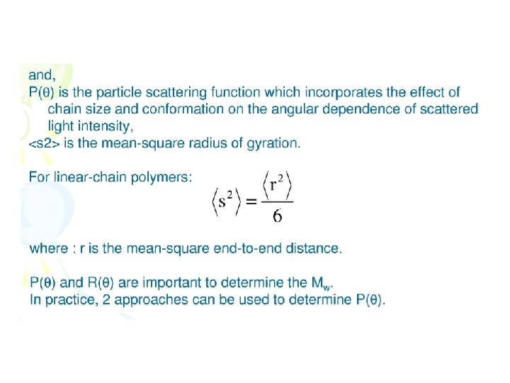
 value, which should be known for all θ values")


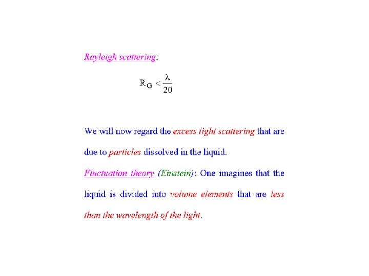

 The concentration fluctuations are also dependent thermo dynamical conditions")
 the size of the particle b) the shape of the particle c) interactions")

- Slides: 67
DETERMINATION OF MOLECULAR WEIGHT OF POLYMERS
Introduction • Molecular weights of polymers can be determined by chemical or physical methods of functional-group analysis. They are measurement of the colligative properties, light scattering, or ultracentrifugation; or by measurement of dilute-solution viscosity. • Molecular weights can be calculated without reference to callibration by another method. Dilute-solution viscosity is not a direct measure of molecular weight and empirically related to molecular weight for many systems. • All methods require the solubility of polymer, involve extrapolation to infinite dilution, and operate in a Θ solvent in which have ideal-solution behaviour
Methods for determination of molecular weight 1. End-group analysis 2. Colligative property measurement 3. Osmometry Vapour Phase Osmometry Membrane Osmometry 4. Ultracentrifugation 5. Light-scattering methods 6. Solution viscosity and molecular size 7. Gel Permeation Chromatography
Methods for Molecular weight determination • Absolute Methods – Colligative property – Ultracentrifugation – Light scattering technique – End group analysis • Relative Methods ü Viscosity • Fractionation Method ü Gel Permeation Chromatography
Different Molecular Weight using different methods Number average Mn • Colligative Properties • Cryoscopy • Ebulliometry • Vapour Pressure • Osmotic pressure • End group Analysis Viscosity Average • Dilute solution viscosity method Weight Average Mw • Ultracentrifugation/ • sedimentation • Light scattering • GPC
Molecular Weight
End Group Analysis •
END GROUP ANALYSIS • The end-group analysis needs the information about the number of determinable groups per molecule. • This method is not suitable for high molecular weight because the fraction of end groups becomes too small to measured with precision. Condensation polymers : End-group analysis in condensation polymers usually involves chemical methods of analysis for functional groups. Examples: • Carboxyl groups in PET and in polyamides are titrated with base in an alcoholic or phenolic solvent. • Amino groups in PA are titrated with acid • Hydroxyl groups is reacted with a titratable reagent Addition polymers : End-group analysis in addition polymers does not have general procedure because of the variety of type and origin of the end groups. Analysis may be made for initiator, elements, radioactive atoms
Requirement for end group analysis • The method cannot be applied to branched polymers • In a linear polymer there are twice as many end of the chain and groups as polymer molecules • If having different end group, the number of detected end group is average molecular weight • End group analysis could be applied for polymerization mechanism identified
Colligative properties • The relations between the colligative properties and molecular weight for infinitely dilute solutions in a fact that the activity of the solute in a solution becomes equal to its mole fraction as the solute concentration becomes sufficiently small. • This method is based on: – Vapour-pressure lowering, – Boiling-point elevation (ebulliometry), – Freezing-point depression (cryoscopy), and – Osmotic pressure (osmometry).
Ebulliometry • In boiling point elevation method the boiling point of the polymer solution is compared directly with that of the pure solvent in a vessel known as ebulliometer. • Sensing device include differential thermometer and multi-junction thermocouples or thermistors in wheat stone bridge circuit. • It is calibrated with a substance of known molecular weight for eg, octacosone M=396 or tristearin M=892 • Accurate molecular weights can be made to 30, 000 • The polymer solutions boil on boiling and can lead to unstable operations • No equipments are suitable for ebulliometry in the high polymer range is commercially available • It is a reference technique and the temperature are to the order of 10⁻³ ºC
Cryoscopy • The freezing point depression or cryoscopic method is similar to the ebullimetric method in several aspects • The preferred temperature-sensing element is a thermistor in a bridge circuit. • The freezing points of solvent and solution are compared sequentially. • Calibration with a substance of known molecular weight is customary • The supercooling needs to be controlled • Molecular weights up-to 30, 000 • Lack of commercial equipments.
Equations Used
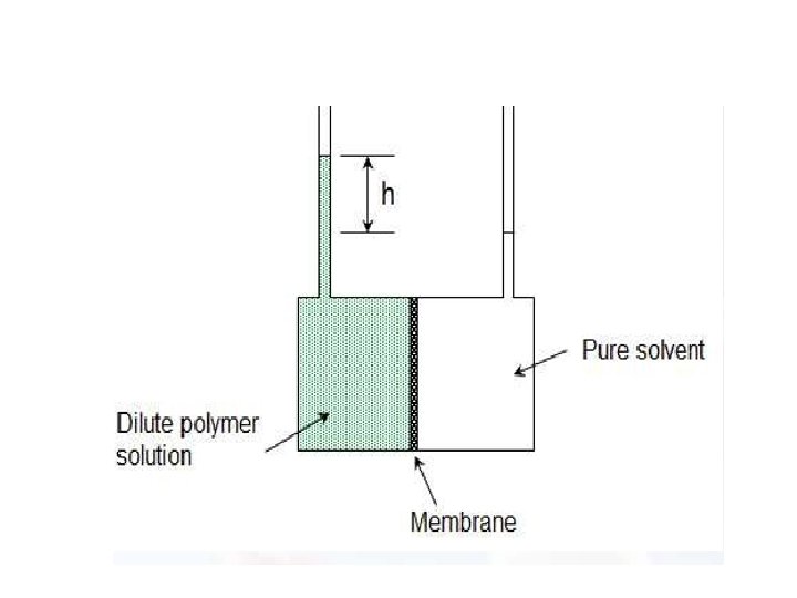
Osmometry • The experimental procedures to determine osmotic pressure are relatively simple but very time consuming. A pure solvent and a dilute solution of the polymer in the same solvent are placed on opposite sides of a semipermeable membrane (cellulose or a cellulose derivative). The differences chemical potentials between solvent and the polymer solution causes solvent to pass through the membrane and raise the liquid head of the solution reservoir. • In the equilibrium pressure: • π= ρgh where ρ is the solvent density.
Osmometry • A basic equation for a solvent:
Osmomerty challenges • Simple experimental procedure, but can be very time consuming • Performance of the membrane can be a problem • Membrane can let some smaller polymer molecules through and this will result in an artificially-higher Mn value • Thus, the method is considered accurate for molecular weights above 20, 000 g/mol • The practical range of molecular weights that can be measured by membrane osmometry is approximately 30000 to one million • For measurements of Mn less than 30000 another technique known as vapour-phase osmometry is more suitable
Vapour Phase Osmometry • Vapor Phase Osmometry is based on the equilibrium thermodynamics of vapor pressure • Vapor Pressure is a colligative property • The determination of Mn operates on the principle that the vapor pressure of a solution is lower than that of the pure solvent at the same temperature and pressure • Magnitude of the vapor pressure decrease is directly proportional to the molar concentration of solute • Does not directly measure vapor pressure but measures change in voltage which is proportional to change in temperature
Introduction • Vapor Phase Osmometry is based on the equilibrium thermodynamics of vapor pressure • Vapor Pressure is a colligative property Vapours
Vapour Phase Osmometry •
The wick provides a vapor saturated atmosphere • Syringes used to inject standard and sample • Thermistors detect changes in temperature • Voltage changes are recorded • System at an equilibrated temperature
Procedure Calibration curve V G/mol • Calibration with standards is necessary – Must have VP no more than 0. 1% of that of the solvent – High Solubility • Common solvents are: – Sucrose octaacetate for organic solution – Simple sucrose for aqueous solution C g/mol Best fit line extrapolated to zero
Molecular weight Determination •
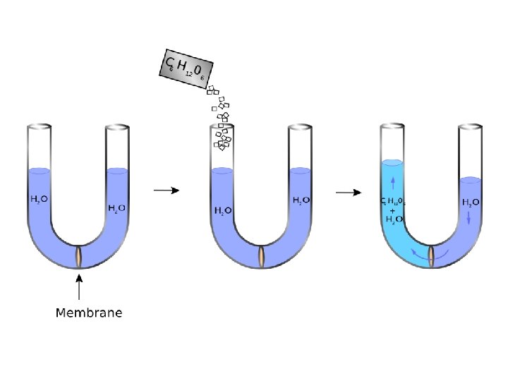
Membrane Osmometry • Osmotic measurements use a semipermeable membrane through which the solvent can freely pass but which excludes polymer molecules. • If this membrane separates two compartments, one filled with pure solvent and the other with a polymer solution, the activity of the solvent in the two compartments is different. • A membrane osmometer is a device used to indirectly measure the number average molecular weight Mn of a polymer sample. • One chamber contains pure solvent and the other chamber contains a solution in which the solute is a polymer with an unknown Mn • The osmotic pressure of the solvent across the semipermeable membrane is measured by the membrane osmometer. • This osmotic pressure measurement is used to calculate Mn for the sample.
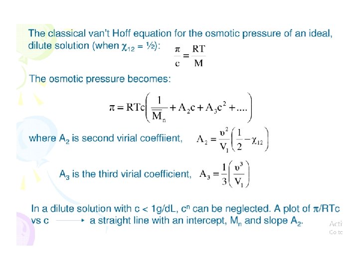
Membrane osmometer: Basic operation • A low concentration solution is created by adding a small amount of polymer to a solvent. • This solution is separated from pure solvent by a semipermeable membrane. • Solute cannot cross the semipermeable membrane but the solvent is able to cross the membrane. • Solvent flows across the membrane to dilute the solution. • The pressure required to stop the flow across the membrane is called the osmotic pressure. • The osmotic pressure is measured and used to calculate Mn In practice, the osmotic pressure produced by an ideally dilute solution would be too small to be accurately measured. For accurate Mn measurements, solutions are not ideally dilute and a virial equation is used to account for deviations from ideal behavior and allow the calculation of Mn
Conclusion Advantages of VPO include: –Speed • Isothermal distillation & Ebullioscopy are slow –Accuracy • Cryoscopy has typical standard deviation of ~10% –Small amount of sample required • Ebullioscopy requires relatively large amount of sample –Useful for a wide range of temperatures • Cryoscopy & Ebullioscopy less flexible Disadvantages of VPO include: – Requires calibration However, Membrane Osmometry does not require calibration – Molecular weight constraints
Ultracentrifugation • A centrifuge is a device for separating particles from a solution according to their size, shape , density, viscosity of medium and rotor speed • Through rapid spinning particles, or even molecules in solution and causes separation of such matter in solution and causes separations of such matter on the basis of differences in weight • Its rotational speed is upto 1, 50, 000 rpm • It creates centrifugal force upto 900, 000 g • The particles are acted on by three forces: Fc The centrifugal force FB Buoyant forces Ff the frictional force between the particle and the liquid • Equation that describes the motion pf this particle as follows F= ma Where m is the mass of the particle and a is the acceleration
The Physics of Ultracentrifugation •
The Physics of Ultracentrifugation •
Sedimentation rate •
Sedimentation Coefficient •
Ultracentrifugation • Stokes equation • Frictional coefficient f=6πȠr� Where: Ƞ-viscosity of solution; r�-particle radius • f is minimal when particle is a sphere • Non- spherical particle has a larger surface area and thus greater value of f.
Types of ultracentrifugation • Used For Analytical centrifugation – To study molecular interactions between macromolecules or to analyse the properties of sedimenting particles such as their apparent molecular weight • Preparative ultracentrifugation : to isolate and purify specific particles
Analytical Centrifugation • Two kinds of experiments are formed: • Sedimentation velocity - To estimate sample purity - Aims to interpret the entire course of sedimentation and report on the shape and molar mass of the dissolved macromolecules, as their size distribution - Components observed as peaks • Sedimentation equilibrium – Only concerned with steady state of the experiment, where sedimentation is balanced by diffusion opposing the concentration gradients, resulting in a time-independent concentration profile
Sedimentation Velocity (Mn)-Sv. • Known concentration of solution is taken solution Solvent • x₁ Time t 1 Direction of the centrifugal force t₂ • x₂ Distance U= X 2 -X 1/ t 2 -t 1 • t₃ x₃ U-sedimentation velocity per unit time Boundary Axis of rotation • S Sₒ c Sₒ-sedimentation coefficient constant Time taken for travel is t 2 and t 1 S= U/ω²(2/X 1+X 2) (sedimentation coefficient) Mn=SₒRT/ Dₒ(1 -ρv) (sevedberg equation) ρ-=density V-molar volume Dₒ= Diffusion constant ω= angular velocity – 65000 rev/min
Sedimentation Equilibrium(SE) Low molecular weight High molecular weight Direction of the centrifugal force X 1 Ca Cb Cc X 2 Axis of rotation X 3
Sedimentation equilibrium (SE)-Mw • 15000 rev/min • S=D (Rate of Sedimentation is equal to rate of diffusion) • (It takes several days to achieve this equilibrium) • The molecular weight which is high is at the bottom). • Mw= 2 RTln(Ca/Cb)/(ω²(1 -ρv)(X 1²-X 2²) • The concentration can be found using other methods like turbidimetric method) • It takes more time • We get the weight average molecular weight by this method
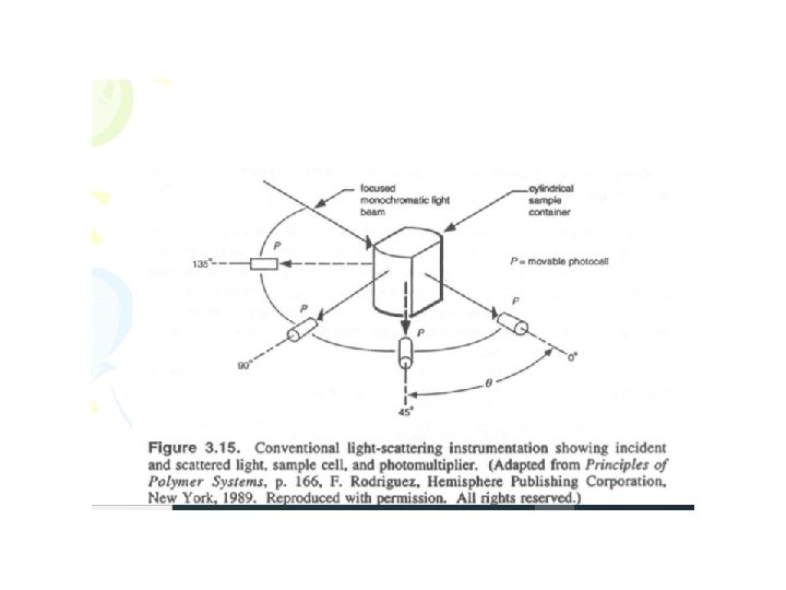
Light Scattering Technique • When light passes through matter, most of the light continues in its original direction but a small fraction is scattered in other directions • Scattered light is proportional to the concentration and molecular weight of the polymer
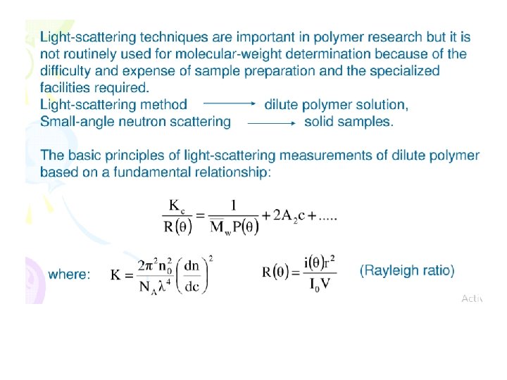
Light Scattering • The weight average molecular weight can be obtained directly only by scattering experiments • Most commonly used is light scattering from dilute polymer solution • Polymer molecules in solution cause stronger scattering than solvent molecules • The intensity of the light is proportionate to the absolute molecular weight of the particle causing the scattering
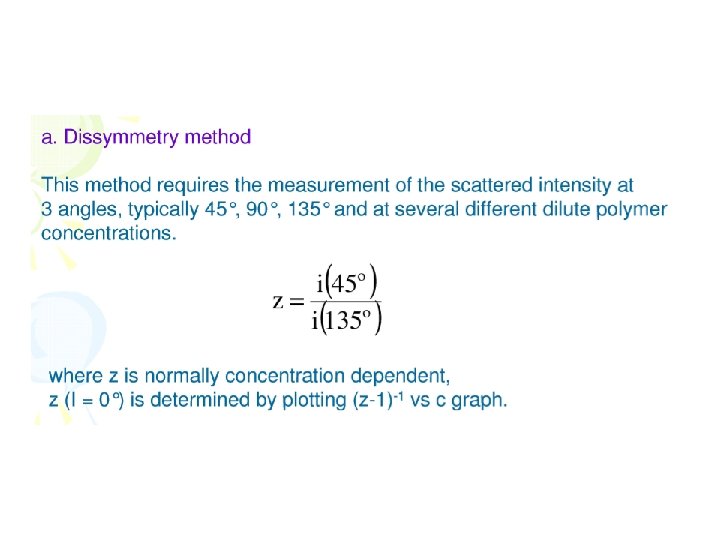
Light Scattering Procedure • Polymer is dissolved in appropriate solvent • The particles have interactions in solution and self organize – Local changes in concentration and density in solution • Light scattering is observed in different angles • Measurements with several concentrations and angles
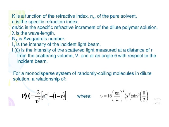
Light Scattering • In order to determine molecular weight, the following information must be known/determined: - Refractive index for the solvent – Difference between refractive indices for the solution and solvent – Polymer concentration – Absolute light intensity for certain scattering angles
Problem is determining R(θ) value, which should be known for all θ values
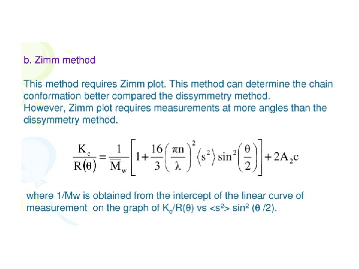
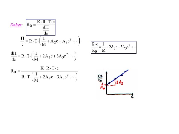
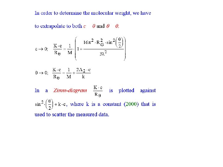
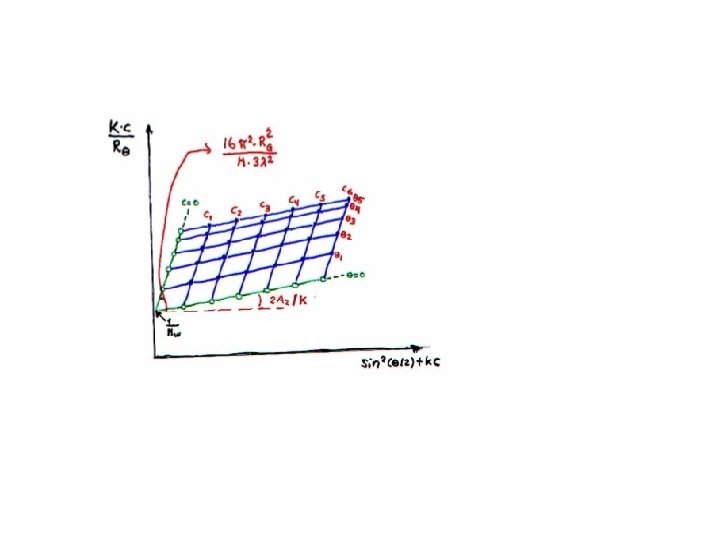
Zimm Plot
Light Scattering
Explanation of Light scattering
r = distance from the particle to the point of observation φ = the angle between the axis of polarization and the direction of the scattered light.
For unpolarized light the analogue expression is:
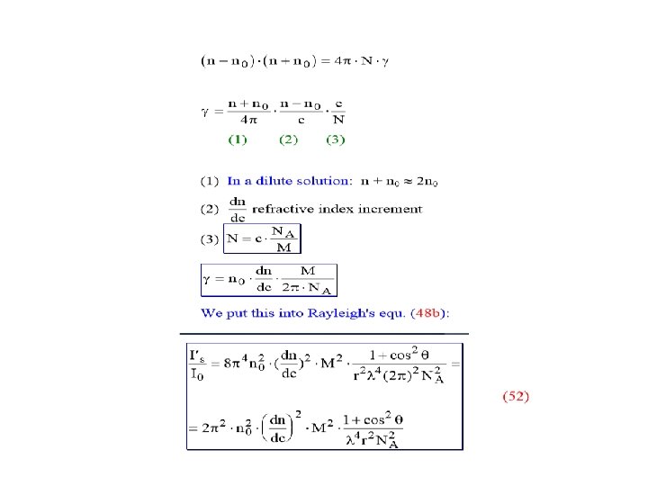
refractive index of solvent and solution, respectively. .
Real solution (at normal concentrations) The concentration fluctuations are also dependent thermo dynamical conditions in the solution.
a) the size of the particle b) the shape of the particle c) interactions between the particles d) the size distribution of the particles
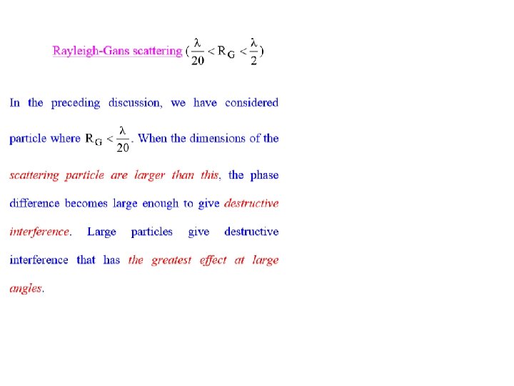
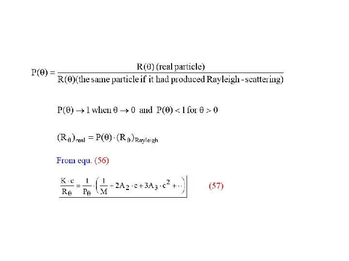
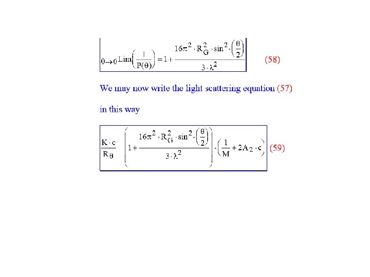
At low scattering angles, θ, and at low concentrations, the angular dependency is independent of the shape of the particle and only dependent on the average radius of gyration of the particle. In practical treatment of light scattering data, we define a function P(θ) = the particlescattering factor or the form factor.