Regression Correlation Time Series Analysis Correlation Analysis is

(Regression, Correlation, Time Series) Analysis

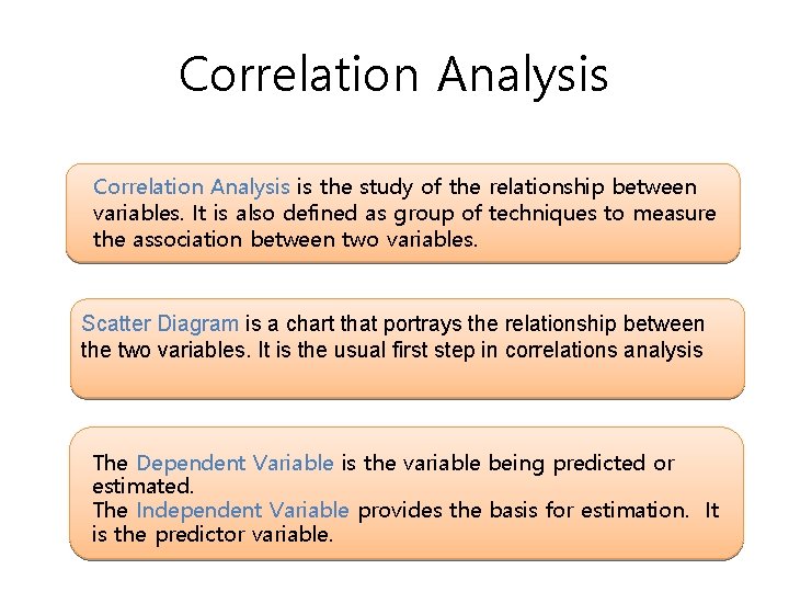
Correlation Analysis is the study of the relationship between variables. It is also defined as group of techniques to measure the association between two variables. Scatter Diagram is a chart that portrays the relationship between the two variables. It is the usual first step in correlations analysis The Dependent Variable is the variable being predicted or estimated. The Independent Variable provides the basis for estimation. It is the predictor variable.

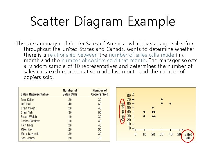
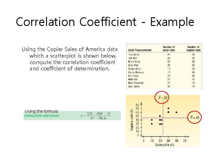
Scatter Diagram Example The sales manager of Copier Sales of America, which has a large sales force throughout the United States and Canada, wants to determine whethere is a relationship between the number of sales calls made in a month and the number of copiers sold that month. The manager selects a random sample of 10 representatives and determines the number of sales calls each representative made last month and the number of copiers sold.

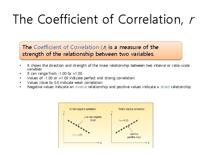
The Coefficient of Correlation, r The Coefficient of Correlation (r) is a measure of the strength of the relationship between two variables. • • • It shows the direction and strength of the linear relationship between two interval or ratio-scale variables It can range from -1. 00 to +1. 00. Values of -1. 00 or +1. 00 indicate perfect and strong correlation. Values close to 0. 0 indicate weak correlation. Negative values indicate an inverse relationship and positive values indicate a direct relationship.

Correlation Coefficient - Example Using the Copier Sales of America data which a scatterplot is shown below, compute the correlation coefficient and coefficient of determination. Using the formula:

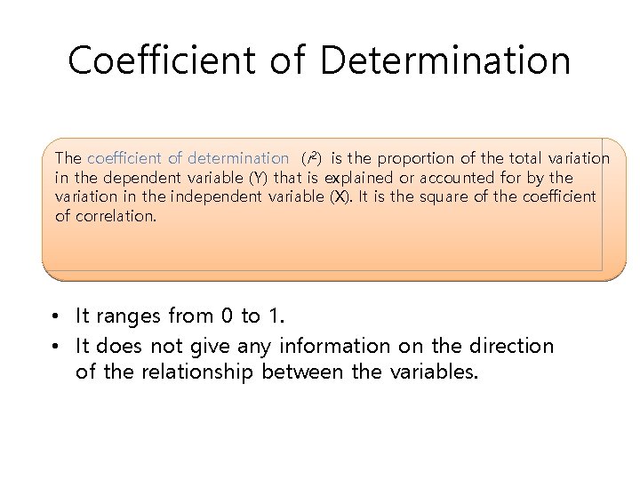
Coefficient of Determination The coefficient of determination (r 2) is the proportion of the total variation in the dependent variable (Y) that is explained or accounted for by the variation in the independent variable (X). It is the square of the coefficient of correlation. • It ranges from 0 to 1. • It does not give any information on the direction of the relationship between the variables.

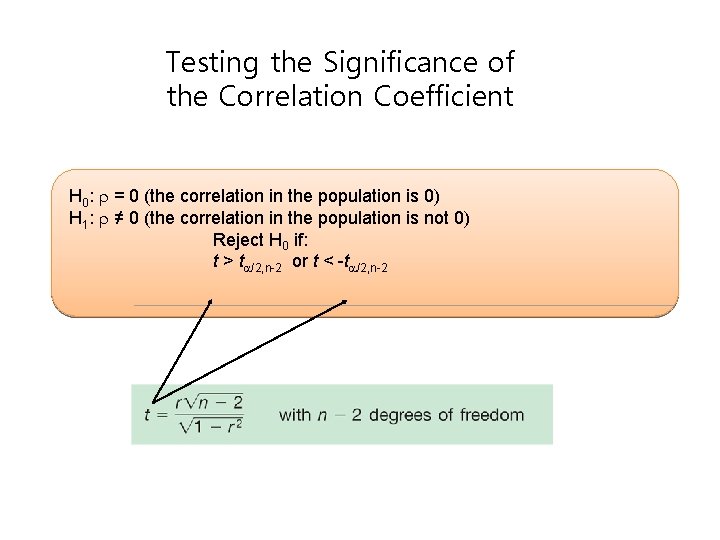
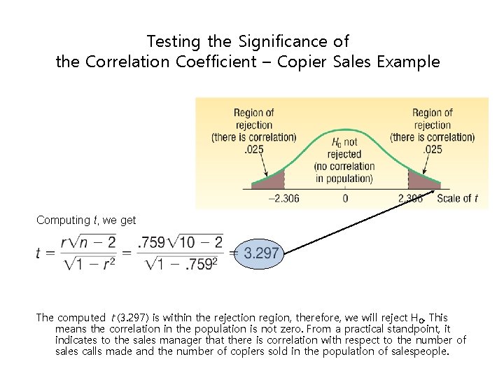
Testing the Significance of the Correlation Coefficient H 0: = 0 (the correlation in the population is 0) H 1: ≠ 0 (the correlation in the population is not 0) Reject H 0 if: t > t /2, n-2 or t < -t /2, n-2

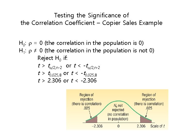
Testing the Significance of the Correlation Coefficient – Copier Sales Example H 0: = 0 (the correlation in the population is 0) H 1: ≠ 0 (the correlation in the population is not 0) Reject H 0 if: t > t /2, n-2 or t < -t /2, n-2 t > t 0. 025, 8 or t < -t 0. 025, 8 t > 2. 306 or t < -2. 306

Testing the Significance of the Correlation Coefficient – Copier Sales Example Computing t, we get The computed t (3. 297) is within the rejection region, therefore, we will reject H 0. This means the correlation in the population is not zero. From a practical standpoint, it indicates to the sales manager that there is correlation with respect to the number of sales calls made and the number of copiers sold in the population of salespeople.

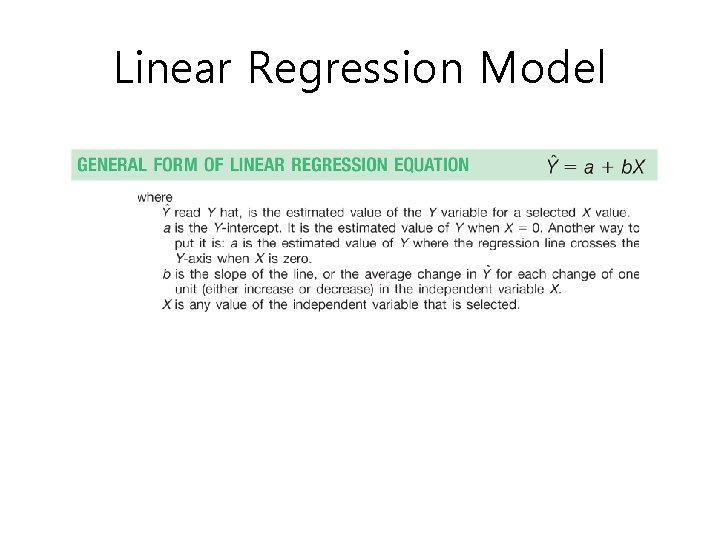
Linear Regression Model

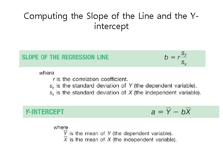
Computing the Slope of the Line and the Yintercept

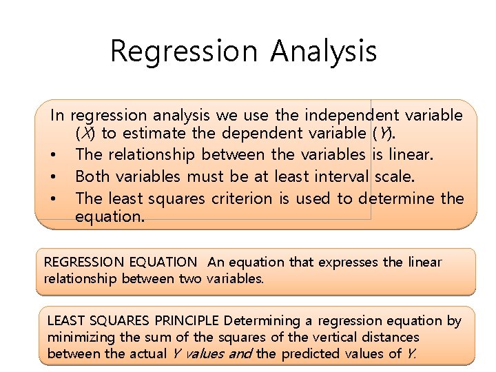
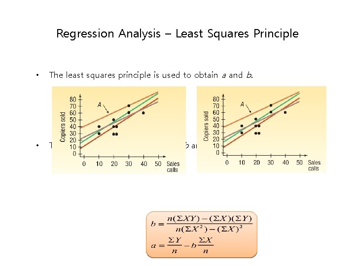
Regression Analysis In regression analysis we use the independent variable (X) to estimate the dependent variable (Y). • The relationship between the variables is linear. • Both variables must be at least interval scale. • The least squares criterion is used to determine the equation. REGRESSION EQUATION An equation that expresses the linear relationship between two variables. LEAST SQUARES PRINCIPLE Determining a regression equation by minimizing the sum of the squares of the vertical distances between the actual Y values and the predicted values of Y.

Regression Analysis – Least Squares Principle • The least squares principle is used to obtain a and b. • The equations to determine a and b are:

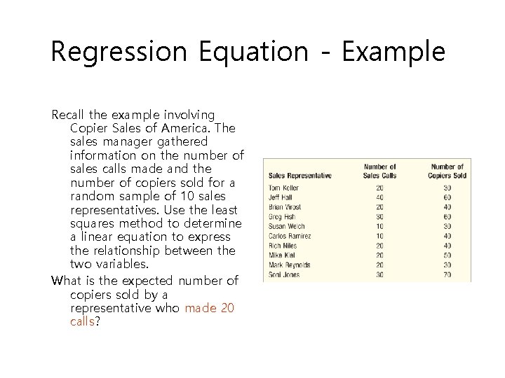
Regression Equation - Example Recall the example involving Copier Sales of America. The sales manager gathered information on the number of sales calls made and the number of copiers sold for a random sample of 10 sales representatives. Use the least squares method to determine a linear equation to express the relationship between the two variables. What is the expected number of copiers sold by a representative who made 20 calls?

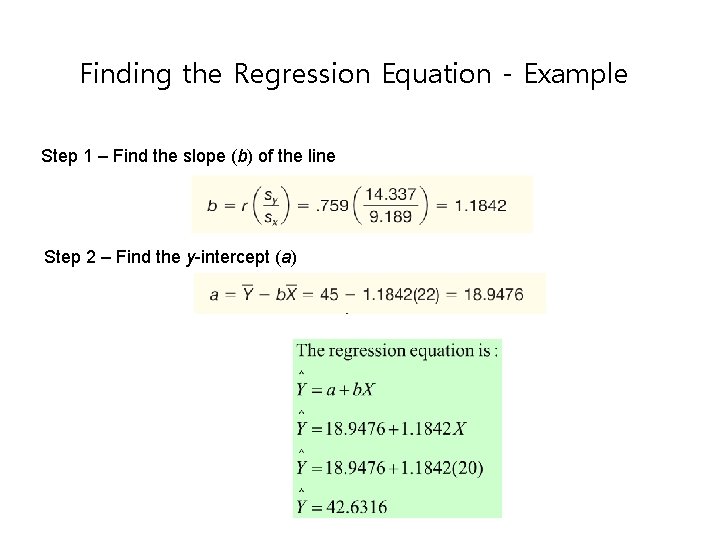
Finding the Regression Equation - Example Step 1 – Find the slope (b) of the line Step 2 – Find the y-intercept (a)

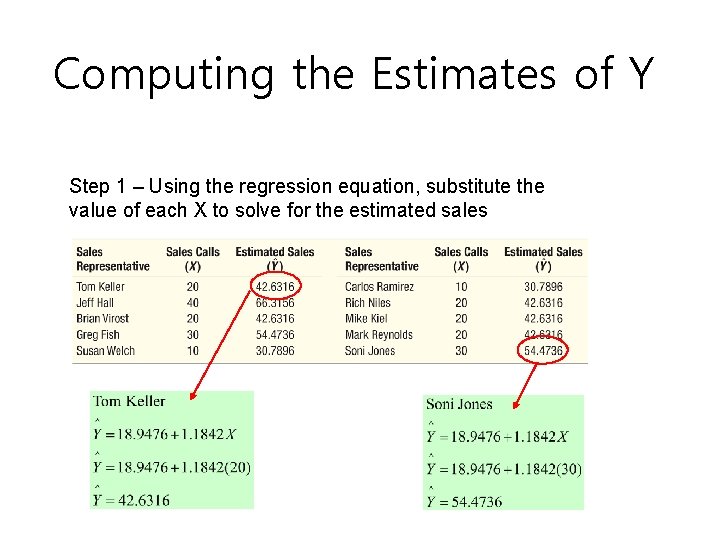
Computing the Estimates of Y Step 1 – Using the regression equation, substitute the value of each X to solve for the estimated sales

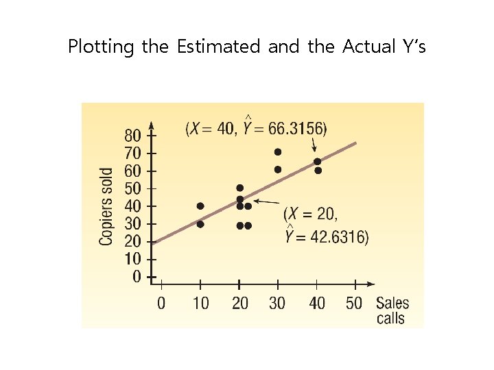
Plotting the Estimated and the Actual Y’s

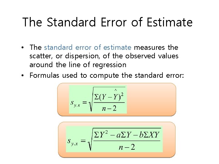
The Standard Error of Estimate • The standard error of estimate measures the scatter, or dispersion, of the observed values around the line of regression • Formulas used to compute the standard error:

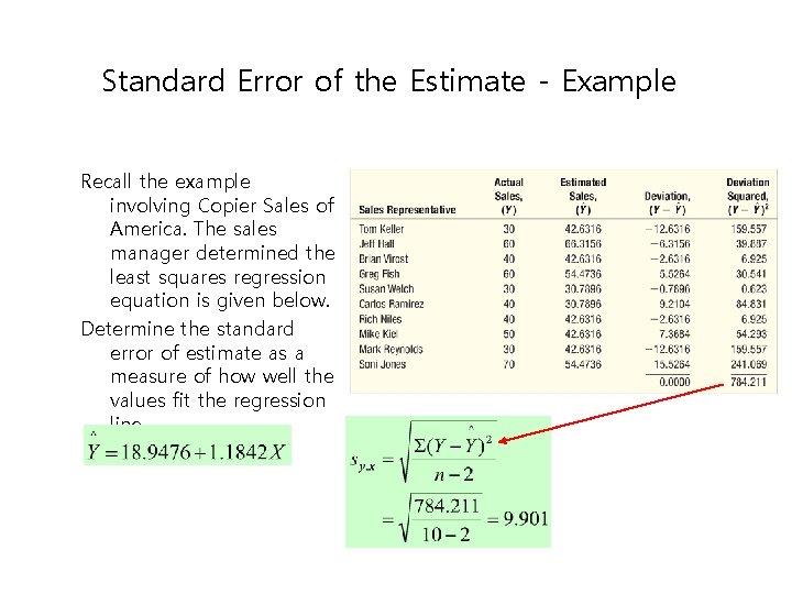
Standard Error of the Estimate - Example Recall the example involving Copier Sales of America. The sales manager determined the least squares regression equation is given below. Determine the standard error of estimate as a measure of how well the values fit the regression line.

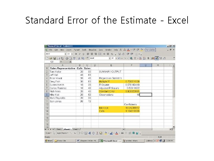
Standard Error of the Estimate - Excel

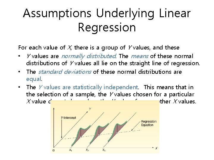
Assumptions Underlying Linear Regression For each value of X, there is a group of Y values, and these • Y values are normally distributed. The means of these normal distributions of Y values all lie on the straight line of regression. • The standard deviations of these normal distributions are equal. • The Y values are statistically independent. This means that in the selection of a sample, the Y values chosen for a particular X value do not depend on the Y values for any other X values.

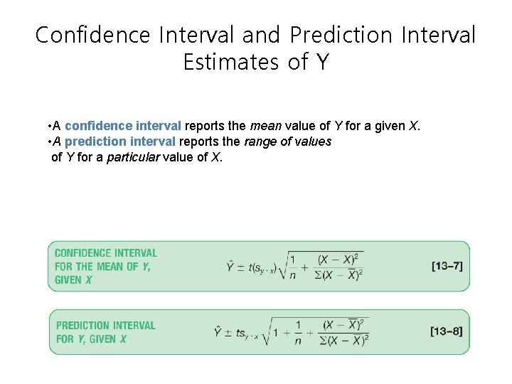
Confidence Interval and Prediction Interval Estimates of Y • A confidence interval reports the mean value of Y for a given X. • A prediction interval reports the range of values of Y for a particular value of X.

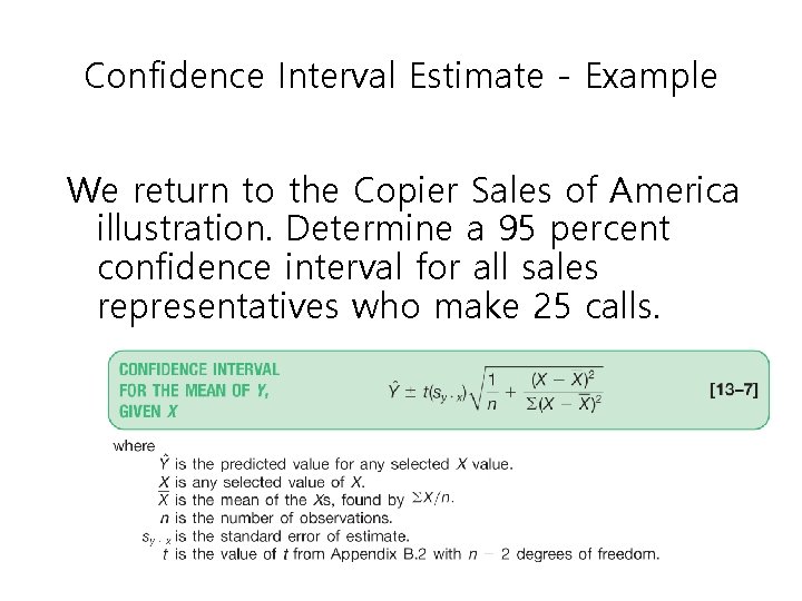
Confidence Interval Estimate - Example We return to the Copier Sales of America illustration. Determine a 95 percent confidence interval for all sales representatives who make 25 calls.

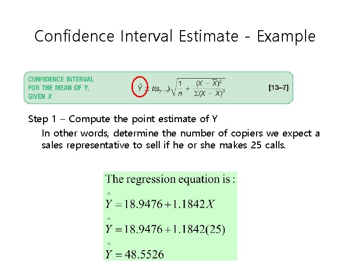
Confidence Interval Estimate - Example Step 1 – Compute the point estimate of Y In other words, determine the number of copiers we expect a sales representative to sell if he or she makes 25 calls.

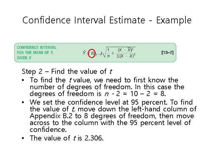
Confidence Interval Estimate - Example Step 2 – Find the value of t • To find the t value, we need to first know the number of degrees of freedom. In this case the degrees of freedom is n - 2 = 10 – 2 = 8. • We set the confidence level at 95 percent. To find the value of t, move down the left-hand column of Appendix B. 2 to 8 degrees of freedom, then move across to the column with the 95 percent level of confidence. • The value of t is 2. 306.

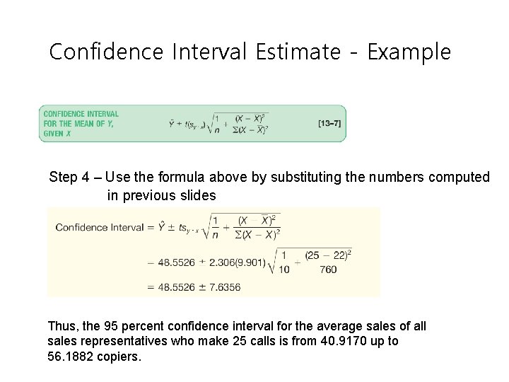
Confidence Interval Estimate - Example Step 4 – Use the formula above by substituting the numbers computed in previous slides Thus, the 95 percent confidence interval for the average sales of all sales representatives who make 25 calls is from 40. 9170 up to 56. 1882 copiers.

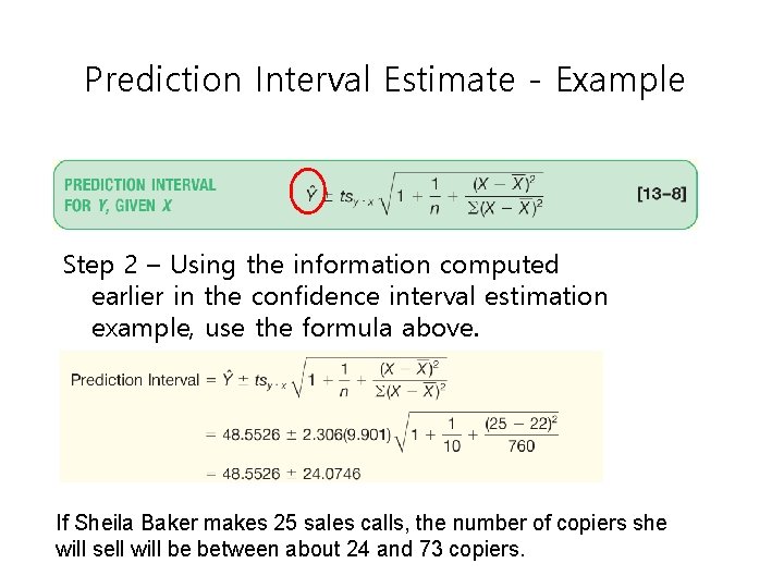
Prediction Interval Estimate - Example We return to the Copier Sales of America illustration. Determine a 95 percent prediction interval for Sheila Baker, a West Coast sales representative who made 25 calls.

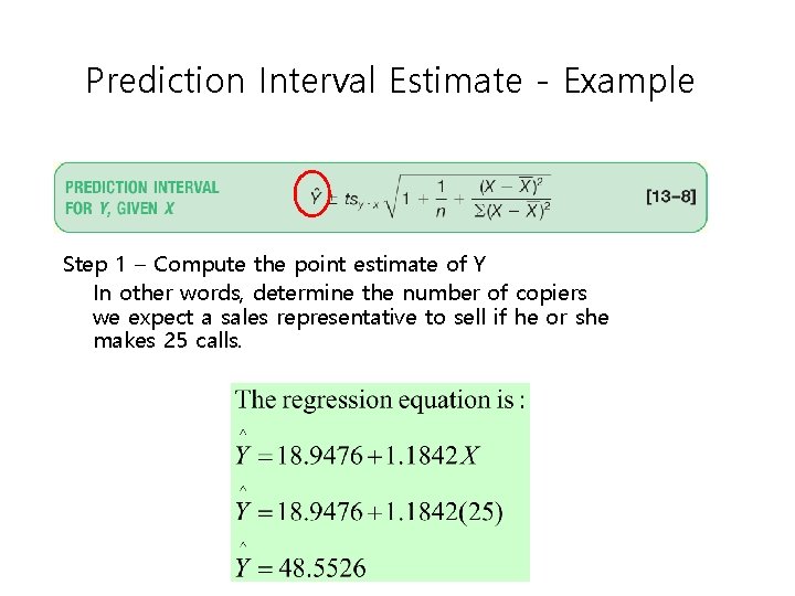
Prediction Interval Estimate - Example Step 1 – Compute the point estimate of Y In other words, determine the number of copiers we expect a sales representative to sell if he or she makes 25 calls.

Prediction Interval Estimate - Example Step 2 – Using the information computed earlier in the confidence interval estimation example, use the formula above. If Sheila Baker makes 25 sales calls, the number of copiers she will sell will be between about 24 and 73 copiers.

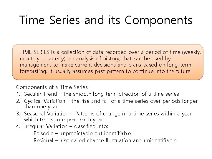
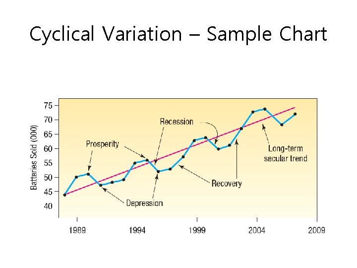
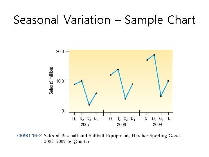
Time Series and its Components TIME SERIES is a collection of data recorded over a period of time (weekly, monthly, quarterly), an analysis of history, that can be used by management to make current decisions and plans based on long-term forecasting. It usually assumes past pattern to continue into the future Components of a Time Series 1. Secular Trend – the smooth long term direction of a time series 2. Cyclical Variation – the rise and fall of a time series over periods longer than one year 3. Seasonal Variation – Patterns of change in a time series within a year which tends to repeat each year 4. Irregular Variation – classified into: Episodic – unpredictable but identifiable Residual – also called chance fluctuation and unidentifiable

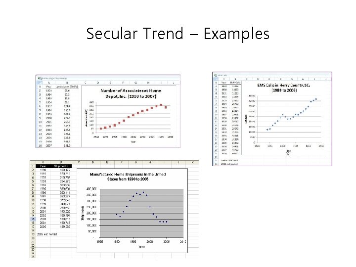
Secular Trend – Examples

Cyclical Variation – Sample Chart

Seasonal Variation – Sample Chart

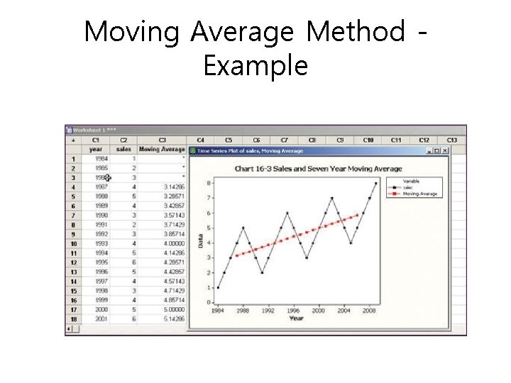
The Moving Average Method • Useful in smoothing time series to see its trend • Basic method used in measuring seasonal fluctuation • Applicable when time series follows fairly linear trend that have definite rhythmic pattern

Moving Average Method Example

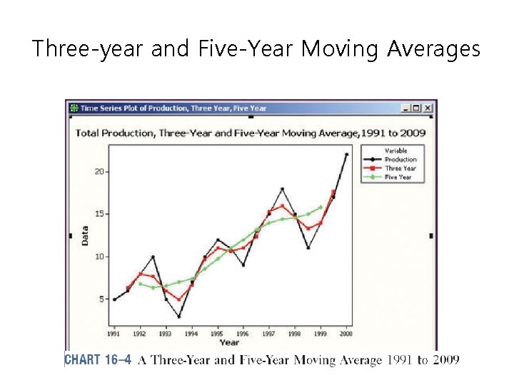
Three-year and Five-Year Moving Averages

Weighted Moving Average • A simple moving average assigns the same weight to each observation in averaging • Weighted moving average assigns different weights to each observation • Most recent observation receives the most weight, and the weight decreases for older data values • In either case, the sum of the weights = 1

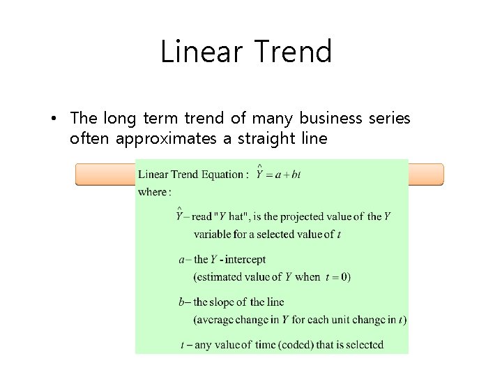
Linear Trend • The long term trend of many business series often approximates a straight line

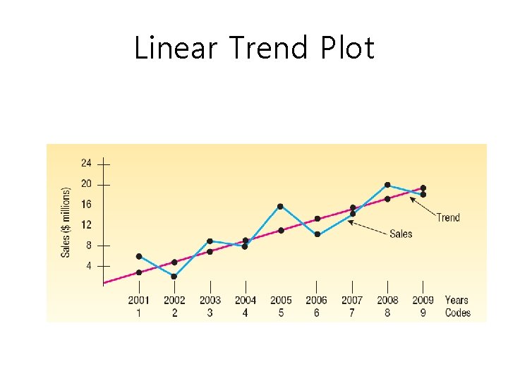
Linear Trend Plot

Linear Trend – Using the Least Squares Method • Use the least squares method in Simple Linear Regression (Chapter 13) to find the best linear relationship between 2 variables • Code time (t) and use it as the independent variable • E. g. let t be 1 for the first year, 2 for the second, and so on (if data are annual)

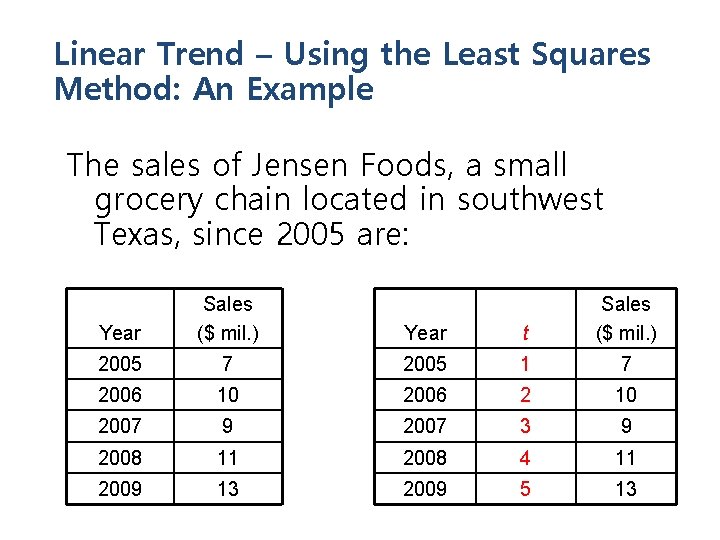
Linear Trend – Using the Least Squares Method: An Example The sales of Jensen Foods, a small grocery chain located in southwest Texas, since 2005 are: Year Sales ($ mil. ) Year t Sales ($ mil. ) 2005 7 2005 1 7 2006 10 2006 2 10 2007 9 2007 3 9 2008 11 2008 4 11 2009 13 2009 5 13

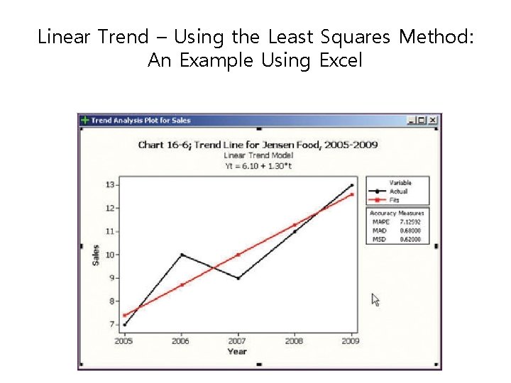
Linear Trend – Using the Least Squares Method: An Example Using Excel

Nonlinear Trends • A linear trend equation is used when the data are increasing (or decreasing) by equal amounts • A nonlinear trend equation is used when the data are increasing (or decreasing) by increasing amounts over time • When data increase (or decrease) by equal percents or proportions plot will show curvilinear pattern

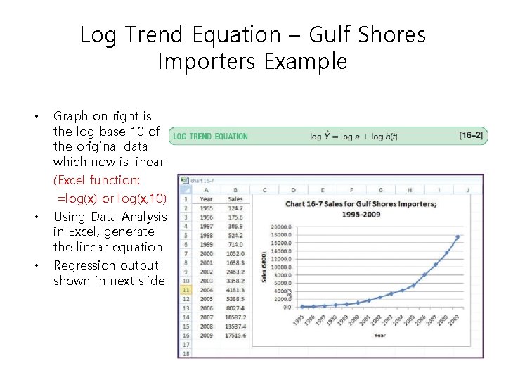
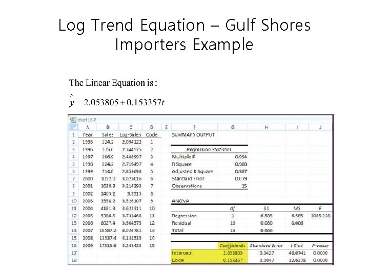
Log Trend Equation – Gulf Shores Importers Example • • • Graph on right is the log base 10 of the original data which now is linear (Excel function: =log(x) or log(x, 10) Using Data Analysis in Excel, generate the linear equation Regression output shown in next slide

Log Trend Equation – Gulf Shores Importers Example

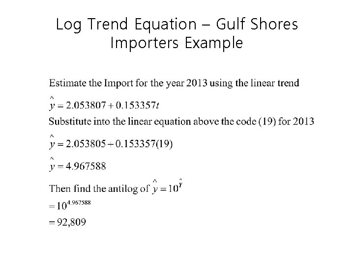
Log Trend Equation – Gulf Shores Importers Example

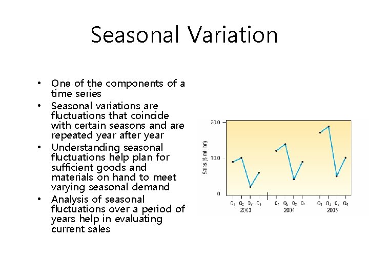
Seasonal Variation • One of the components of a time series • Seasonal variations are fluctuations that coincide with certain seasons and are repeated year after year • Understanding seasonal fluctuations help plan for sufficient goods and materials on hand to meet varying seasonal demand • Analysis of seasonal fluctuations over a period of years help in evaluating current sales

Seasonal Index • A number, usually expressed in percent, that expresses the relative value of a season with respect to the average for the year (100%) • Ratio-to-moving-average method – The method most commonly used to compute the typical seasonal pattern – It eliminates the trend (T), cyclical (C), and irregular (I) components from the time series

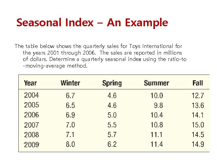
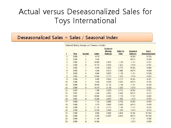
Seasonal Index – An Example The table below shows the quarterly sales for Toys International for the years 2001 through 2006. The sales are reported in millions of dollars. Determine a quarterly seasonal index using the ratio-to -moving-average method.

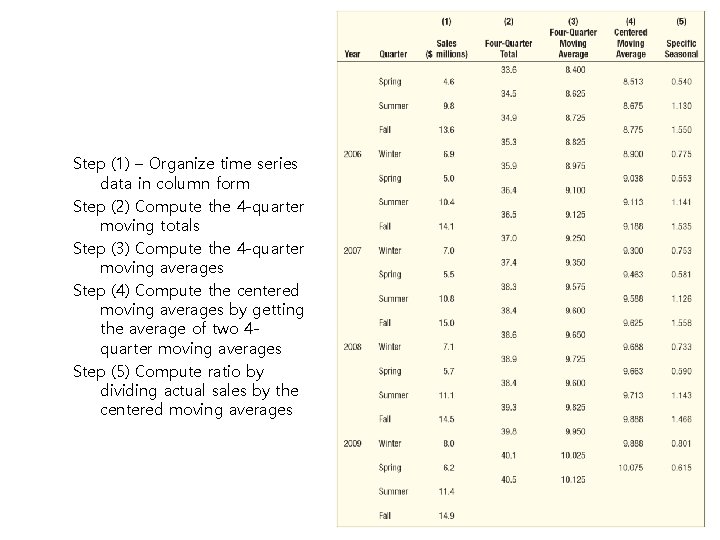
Step (1) – Organize time series data in column form Step (2) Compute the 4 -quarter moving totals Step (3) Compute the 4 -quarter moving averages Step (4) Compute the centered moving averages by getting the average of two 4 quarter moving averages Step (5) Compute ratio by dividing actual sales by the centered moving averages

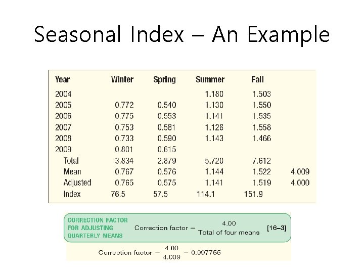
Seasonal Index – An Example

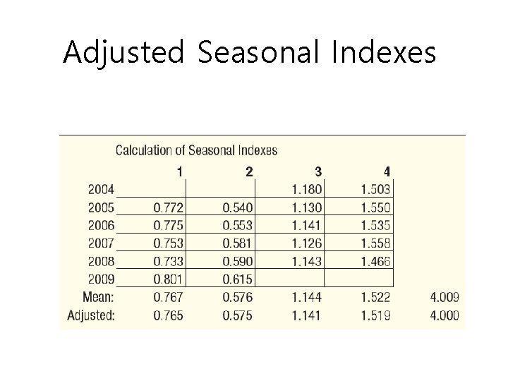
Adjusted Seasonal Indexes

Actual versus Deseasonalized Sales for Toys International Deseasonalized Sales = Sales / Seasonal Index

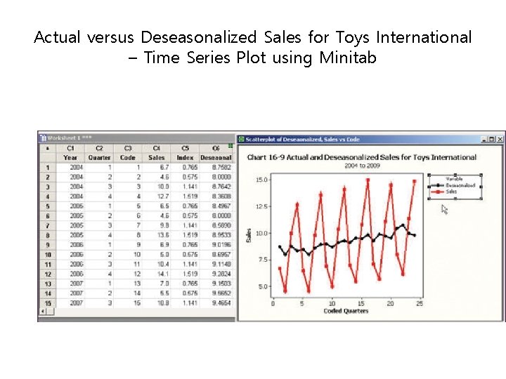
Actual versus Deseasonalized Sales for Toys International – Time Series Plot using Minitab

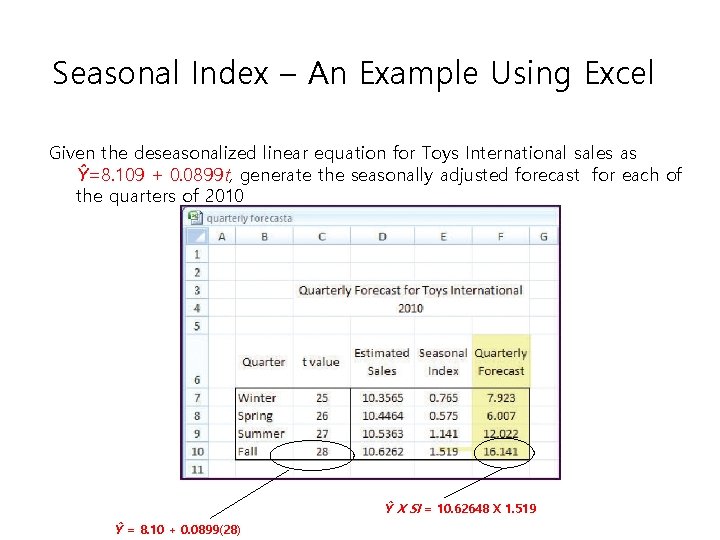
Seasonal Index – An Example Using Excel Given the deseasonalized linear equation for Toys International sales as Ŷ=8. 109 + 0. 0899 t, generate the seasonally adjusted forecast for each of the quarters of 2010 Ŷ X SI = 10. 62648 X 1. 519 Ŷ = 8. 10 + 0. 0899(28)

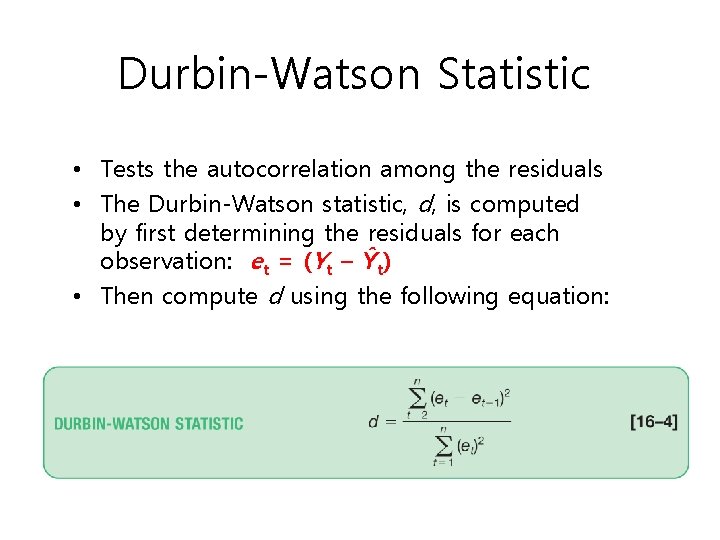
Durbin-Watson Statistic • Tests the autocorrelation among the residuals • The Durbin-Watson statistic, d, is computed by first determining the residuals for each observation: et = (Yt – Ŷt) • Then compute d using the following equation:

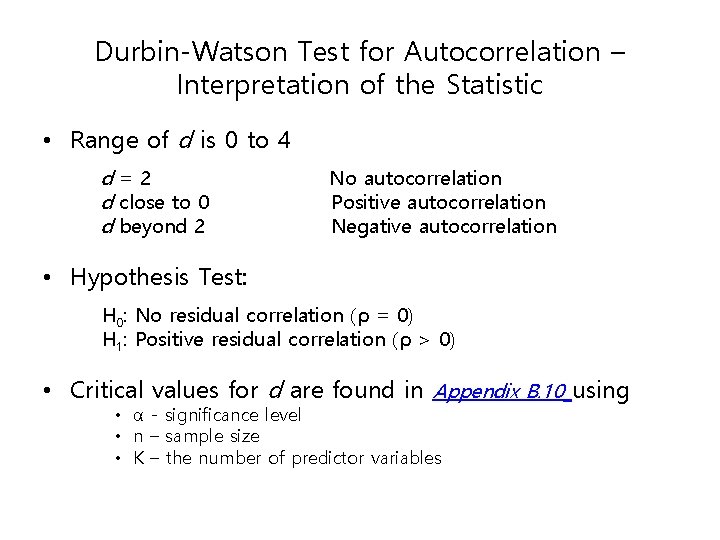
Durbin-Watson Test for Autocorrelation – Interpretation of the Statistic • Range of d is 0 to 4 d=2 d close to 0 d beyond 2 No autocorrelation Positive autocorrelation Negative autocorrelation • Hypothesis Test: H 0: No residual correlation (ρ = 0) H 1: Positive residual correlation (ρ > 0) • Critical values for d are found in Appendix B. 10 using • α - significance level • n – sample size • K – the number of predictor variables

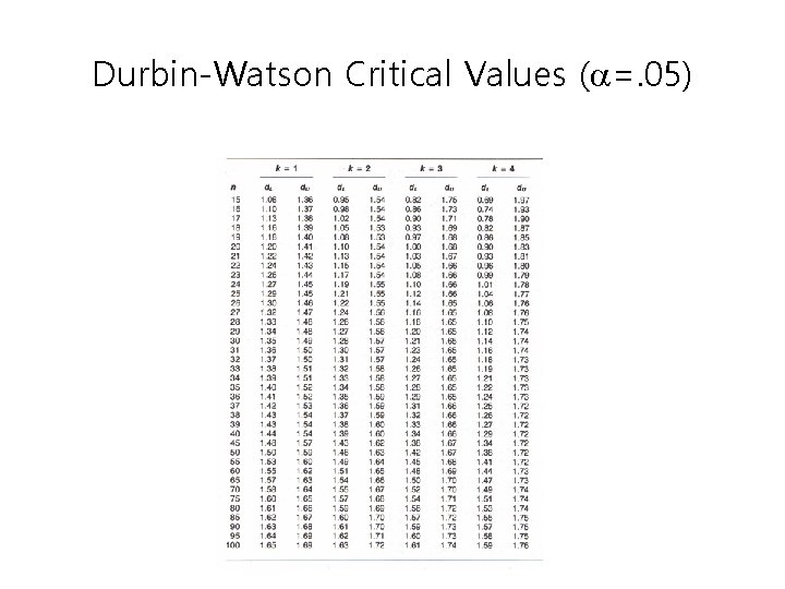
Durbin-Watson Critical Values ( =. 05)

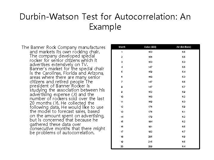
Durbin-Watson Test for Autocorrelation: An Example The Banner Rock Company manufactures and markets its own rocking chair. The company developed special rocker for senior citizens which it advertises extensively on TV. Banner’s market for the special chair is the Carolinas, Florida and Arizona, areas where there are many senior citizens and retired people The president of Banner Rocker is studying the association between his advertising expense (X) and the number of rockers sold over the last 20 months (Y). He collected the following data. He would like to use the model to forecast sales, based on the amount spent on advertising, but is concerned that because he gathered these data over consecutive months that there might be problems of autocorrelation. Month Sales (000) Ad ($millions) 1 153 5. 5 2 156 5. 5 3 153 5. 3 4 147 5. 5 5 159 5. 4 6 160 5. 3 7 147 5. 5 8 147 5. 7 9 152 5. 9 10 160 6. 2 11 169 6. 3 12 176 5. 9 13 176 6. 1 14 179 6. 2 15 184 6. 2 16 181 6. 5 17 192 6. 7 18 205 6. 9 19 215 6. 5 20 209 6. 4

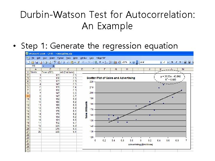
Durbin-Watson Test for Autocorrelation: An Example • Step 1: Generate the regression equation

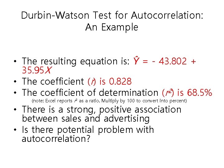
Durbin-Watson Test for Autocorrelation: An Example • The resulting equation is: Ŷ = - 43. 802 + 35. 95 X • The coefficient (r) is 0. 828 • The coefficient of determination (r 2) is 68. 5% (note: Excel reports r 2 as a ratio. Multiply by 100 to convert into percent) • There is a strong, positive association between sales and advertising • Is there potential problem with autocorrelation?

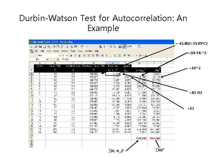
Durbin-Watson Test for Autocorrelation: An Example =-43. 802+35. 95*C 3 =(E 4 -F 4)^2 =E 4^2 =B 3 -D 3 =E 3 ∑(ei -ei-1)2 ∑(ei)2

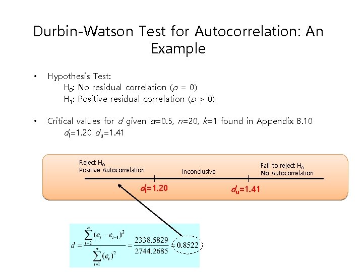
Durbin-Watson Test for Autocorrelation: An Example • Hypothesis Test: H 0: No residual correlation (ρ = 0) H 1: Positive residual correlation (ρ > 0) • Critical values for d given α=0. 5, n=20, k=1 found in Appendix B. 10 dl=1. 20 du=1. 41 Reject H 0 Positive Autocorrelation dl=1. 20 Fail to reject H 0 No Autocorrelation Inconclusive du=1. 41