Group Analysis with AFNI Programs H H Major

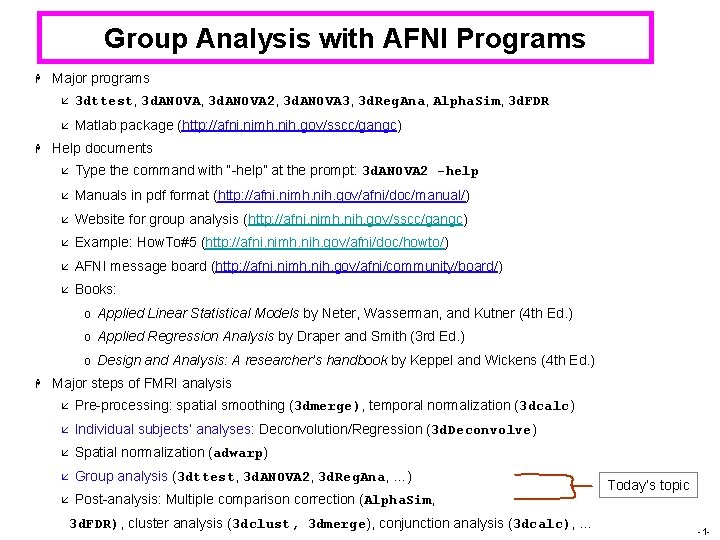
Group Analysis with AFNI Programs H H Major programs å 3 dttest, 3 d. ANOVA 2, 3 d. ANOVA 3, 3 d. Reg. Ana, Alpha. Sim, 3 d. FDR å Matlab package (http: //afni. nimh. nih. gov/sscc/gangc) Help documents å Type the command with “-help” at the prompt: 3 d. ANOVA 2 -help å Manuals in pdf format (http: //afni. nimh. nih. gov/afni/doc/manual/) å Website for group analysis (http: //afni. nimh. nih. gov/sscc/gangc) å Example: How. To#5 (http: //afni. nimh. nih. gov/afni/doc/howto/) å AFNI message board (http: //afni. nimh. nih. gov/afni/community/board/) å Books: o Applied Linear Statistical Models by Neter, Wasserman, and Kutner (4 th Ed. ) o Applied Regression Analysis by Draper and Smith (3 rd Ed. ) o Design and Analysis: A researcher’s handbook by Keppel and Wickens (4 th Ed. ) H Major steps of FMRI analysis å Pre-processing: spatial smoothing (3 dmerge), temporal normalization (3 dcalc) å Individual subjects’ analyses: Deconvolution/Regression (3 d. Deconvolve) å Spatial normalization (adwarp) å Group analysis (3 dttest, 3 d. ANOVA 2, 3 d. Reg. Ana, …) å Post-analysis: Multiple comparison correction (Alpha. Sim, 3 d. FDR), cluster analysis (3 dclust, 3 dmerge), conjunction analysis (3 dcalc), … Today’s topic -1 -

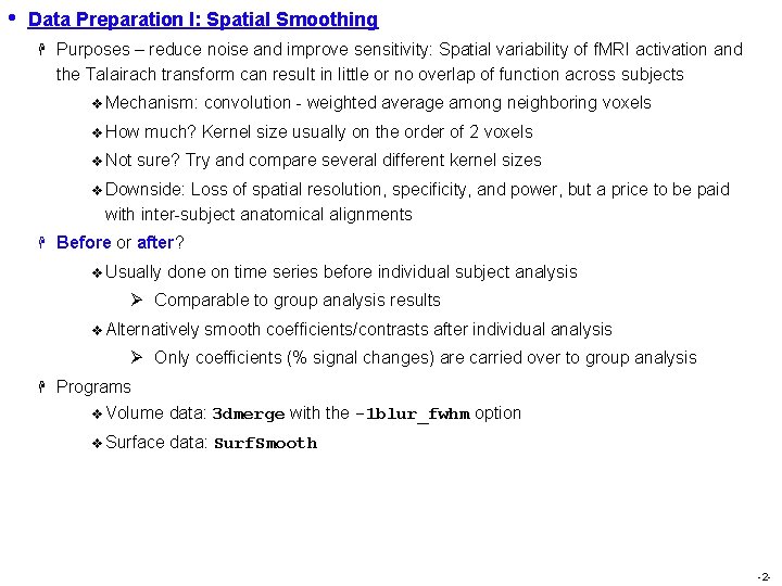
• Data Preparation I: Spatial Smoothing H Purposes – reduce noise and improve sensitivity: Spatial variability of f. MRI activation and the Talairach transform can result in little or no overlap of function across subjects v Mechanism: convolution - weighted average among neighboring voxels v How much? Kernel size usually on the order of 2 voxels v Not sure? Try and compare several different kernel sizes v Downside: Loss of spatial resolution, specificity, and power, but a price to be paid with inter-subject anatomical alignments H Before or after? v Usually done on time series before individual subject analysis Ø Comparable to group analysis results v Alternatively smooth coefficients/contrasts after individual analysis Ø Only coefficients (% signal changes) are carried over to group analysis H Programs v Volume data: 3 dmerge with the -1 blur_fwhm option v Surface data: Surf. Smooth -2 -

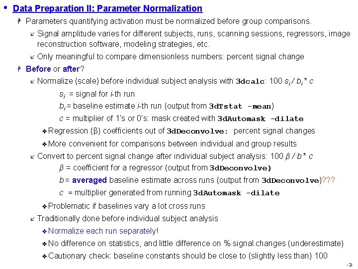
• Data Preparation II: Parameter Normalization H H Parameters quantifying activation must be normalized before group comparisons. å Signal amplitude varies for different subjects, runs, scanning sessions, regressors, image reconstruction software, modeling strategies, etc. å Only meaningful to compare dimensionless numbers: percent signal change Before or after? å Normalize (scale) before individual subject analysis with 3 dcalc: 100 si / bi * c si = signal for i-th run bi = baseline estimate i-th run (output from 3 d. Tstat -mean) c = multiplier of 1’s or 0’s: mask created with 3 d. Automask -dilate v Regression (β) coefficients out of 3 d. Deconvolve: percent signal changes v More convenient for comparisons between individual and group results å Convert to percent signal change after individual subject analysis: 100 β / b * c β = coefficient for a regressor (output from 3 d. Deconvolve) b = averaged baseline estimate across runs (output from 3 d. Deconvolve)? ? ? c = multiplier generated from running 3 d. Automask -dilate v Problematic if baselines vary a lot cross runs å Traditionally done before individual subject analysis v Normalize each run separately! v No difference on statistics, and little difference on % signal changes (underestimate) v Cautionary check: baseline constants should be close to (slightly less than) 100 -3 -

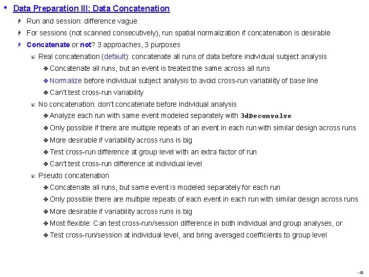
• Data Preparation III: Data Concatenation H Run and session: difference vague H For sessions (not scanned consecutively), run spatial normalization if concatenation is desirable H Concatenate or not? 3 approaches, 3 purposes å Real concatenation (default): concatenate all runs of data before individual subject analysis v Concatenate all runs, but an event is treated the same across all runs v Normalize before individual subject analysis to avoid cross-run variability of base line v Can’t test cross-run variability å No concatenation: don’t concatenate before individual analysis v Analyze each run with same event modeled separately with 3 d. Deconvolve v Only possible if there are multiple repeats of an event in each run with similar design across runs v More desirable if variability across runs is big v Test cross-run difference at group level with an extra factor of run v Can’t test cross-run difference at individual level å Pseudo concatenation v Concatenate all runs, but same event is modeled separately for each run v Only possible there are multiple repeats of each event in each run with similar design across runs v More desirable if variability across runs is big v Most flexible: Can test cross-run/session difference in both individual and group analyses, or v Test cross-run/session at individual level, and bring averaged coefficients to group level -4 -

• Data Preparation IV: Co-Registration (AKA “Spatial Normalization”) H Improve sensitivity: Group analysis on voxel-by-voxel basis; Must be aligned/defined over same domain H Before or after? å Usually done after individual subject analysis v Keep close to the original data v Save huge runtime in 3 d. Deconvolve å Can alternatively done before 3 d. Deconvolve v More desirable for cross-session concatenation v Compare group results with individual activation maps v Before or after, no significant difference in terms of group analysis results v Convert to lower resolution with roughly the same resolution as EPI (adwarp -dxyz) H Steps and programs å Volumetric data v Anatomical data transformation: manual (AFNI) or automatic (@auto_tlrc) v Transform functional data using AFNI interactively or adwarp (use option -dxyz with about the same resolution as EPI data — do not have to use the default 1 mm resolution!) å Surface data: Standard meshes and spherical coordinate system v Surface models of the cortical surface are warped to match a template surface using Caret/Sure. Fit (http: //brainmap. wustl. edu) or Free. Surfer (http: //surfer. nmr. mgh. harvard. edu) v Standard-mesh surface models are then created with SUMA (http: //afni. nimh. nih. gov/ssc/ziad/SUMA) to allow for node-based group analysis å Once data is aligned, analysis is carried out voxel-by-voxel or node-by-node v Analyses and results are on the percent signal changes v Display resulting statistics (voxel-wise or node-wise) AFNI and/or SUMA -5 -

• Basics about null hypothesis significance testing (NHST) H Controversy: Are humans cognitively good intuitive statisticians? H Quiz: HIV prevalence = 10 -3, false + of HIV test = 5%, power of HIV test = 100%. å H P(HIV+ | test+) = ? Cohen, J. , "The Earth Is Round (p <. 05)“ (1994), American Psychologist, 49, 12 997 -1003 å Ritualized dichotomous decisions around a sacred number 0. 05 H H 0: no task effect or no response difference between two tasks at a voxel vs H 1: there is difference H What does it mean with a dichotomous decision and rejecting H 0 at a significant level α (e. g. , 0. 05)? å Conditional probability P(result | H 0) = α, not P(H 0)! å 2 types of errors: type I and type II Ø Type I error = α, Type II error = β = P(accept H 0 | H 1); Power = P(accept H 1 | H 1) = 1 – β Ø Traditional strategy: control type I error while gaining power as much as possible Ø Importance of checking efficiency (power) of your design with RSFgen before scanning Ø Norman H. Anderson: “the main function of statistics is to get more information into the data. " å Usual misinterpretations Ø Reject H 0 ==> Prove or confirm a theory (alternative hypothesis)! (wrong!) Ø P(result | H 0) = P(H 0) (wrong!) Ø P(result | H 0) = Probability if the experiment can be reproduced (wrong!) H Keep in mind å Better plan than sorry: Spend more time on experiment design (power analysis) å More appropriate for detection than sanctification of a theory å Try to avoid unnecessary overstatement when making conclusions å Present graphics and report percent signal change, standard deviation, confidence interval, … å Replications are the best strategy on induction/generalization -6 -

• Quiz: How do you interpret the results of a null hypothesis significance test? A researcher tested the null hypothesis that two population means are equal (H 0: μ 1 = μ 2). A t-test produced p=0. 01. Assuming that all assumptions of the test have been satisfied, which of the following statements are true and which are false? Why? 1. There is a 1% chance of getting a result even more extreme than the observed one when H 0 is true. 2. There is a 1% likelihood that the result happened by chance. 3. There is a 1% chance that the null hypothesis is true. 4. There is a 1% chance that the decision to reject H 0 is wrong. 5. There is a 99% chance that the alternative hypothesis is true, given the observed data. 6. A small p value indicates a large effect. 7. Rejection of H 0 confirms the alternative hypothesis. 8. Failure to reject H 0 means that the two population means are probably equal. 9. Rejecting H 0 confirms the quality of the research design. 10. If H 0 is not rejected, the study is a failure. 11. If H 0 is rejected in Study 1 but not rejected in Study 2, there must be a moderator variable that accounts for the difference between the two studies. 12. There is a 99% chance that a replication study will produce significant results. 13. Assuming H 0 is true and the study is repeated many times, 1% of these results will be even more inconsistent with H 0 than the observed result. Adapted from Kline, R. B. (2004). Beyond significance testing. Washington, DC: American Psychological Association (pp. 63 -69). Dale Berger, CGU 9/04 -7 -

• Basics of Group Analysis H General Linear Model (GLM) and ANOVA H Factor and level H å Dependant and independent variable å Factors: categorizing variables, e. g. , subject category and stimulus class å Levels: nominal (qualitative) values of a factor, e. g. , conditions 1, 2, and 3 Fixed/random factor å Fixed: effects/contrasts at specific levels are of interest å Random (usually subject in f. MRI): each level of the factor is not of interest, but should model variance for generalizing the conclusion to whole population H Factorial (crossed)/nested (more specifically within-subject/between-subjects) design H Different terminology H å count subject as a random factor (statisticians) å within-subject (repeated measures)/between-subjects (psychologists) Group analysis: partition/untangle data variability into various sources å Cell-mean (or structural) model of one-way within-subject ANOVA: Yij = μ + αi+ βj + εij o Yij independent variable, percent signal change of subject j with task i; o μ constant – grand/common mean; o αi constants subject to Σαi = 0 – simple effect of factor A at level i, i = 1, 2, . . . , a; o βj independent N(0, σp 2) – random effect of subject j, j = 1, 2, . . . , b (σp 2 - population variance); o εij independent N(0, σ2) – interaction: within-subject variability (σ2 - variance of sampling error) -8 -

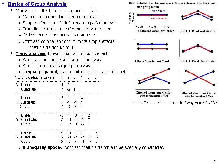
• Basics of Group Analysis H H Main/simple effect, interaction, and contrast Ø Main effect: general info regarding a factor Ø Simple effect: specific info regarding a factor level Ø Disordinal interaction: differences reverse sign Ø Ordinal interaction: one above another Ø Contrast: comparison of 2 or more simple effects; coefficients add up to 0 Trend analysis: Linear, quadratic or cubic effect Ø Among stimuli (individual subject analysis) Ø Among factor levels (group analysis) Ø If equally-spaced, use the orthogonal polynomial coefficients No. of Conditions/Levels 1 2 3 4 5 6 ----------------------------------------------------- 3 Linear -1 0 1 Quadratic 1 -2 1 ----------------------------------------------------- Linear -3 -1 1 3 4 Quadratic 1 -1 1 Cubic -1 3 -3 1 ----------------------------------------------------- Linear -2 -1 0 1 2 5 Quadratic 2 -1 -2 -1 2 Cubic -1 2 0 -2 1 ----------------------------------------------------- Linear -5 -3 -1 1 3 5 6 Quadratic 5 -1 -4 -1 5 Cubic -5 7 4 -7 5 Ø Main effects and interactions in 2 -way mixed ANOVA If unequally-spaced, contrast coefficients have to be specially constructed -9 -

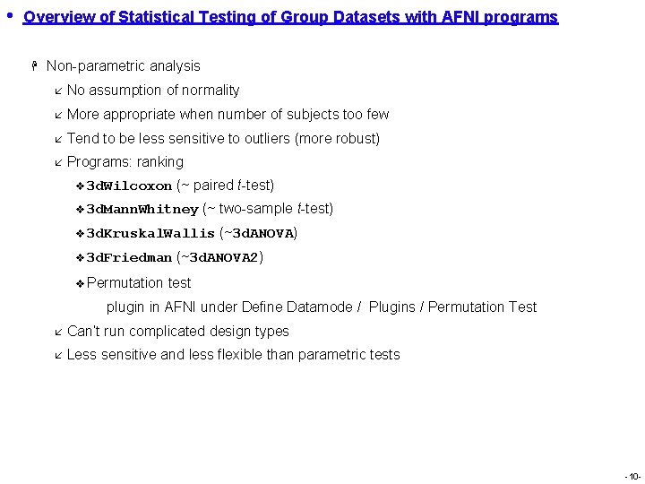
• Overview of Statistical Testing of Group Datasets with AFNI programs H Non-parametric analysis å No assumption of normality å More appropriate when number of subjects too few å Tend to be less sensitive to outliers (more robust) å Programs: ranking v 3 d. Wilcoxon (~ paired t-test) v 3 d. Mann. Whitney (~ two-sample t-test) v 3 d. Kruskal. Wallis (~3 d. ANOVA) v 3 d. Friedman (~3 d. ANOVA 2) v Permutation test plugin in AFNI under Define Datamode / Plugins / Permutation Test å Can’t run complicated design types å Less sensitive and less flexible than parametric tests -10 -

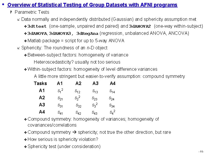
• Overview of Statistical Testing of Group Datasets with AFNI programs H Parametric Tests å Data normally and independently distributed (Gaussian) and sphericity assumption met v 3 dttest (one-sample, unpaired and paired) and 3 d. ANOVA 2 (one-way within-subject) v 3 d. ANOVA, 3 d. ANOVA 3, 3 d. Reg. Ana (regression, unbalanced ANOVA, ANCOVA) v Matlab package = script for up to 5 -way ANOVA å Sphericity: The roundness of an n-D object v Between-subject factors: homogeneity of variance Heteroscedasticity? usually not too serious v Within-subject factors: homogeneity of level difference variances A little more stringent but easier-to-verify assumption: compound symmetry Tasks A 1 A 2 A 3 A 4 A 1 s 12 s 13 s 14 A 2 s 21 s 22 s 23 s 24 A 3 s 31 s 32 s 34 A 4 s 41 s 42 s 43 s 42 v Compound symmetry: homogeneity of variances; homogeneity of covariances/correlations v Compound symmetry sphericity; not true the other direction, but rare v How serious is sphericity violation? v Sphericity test (under consideration) -11 -

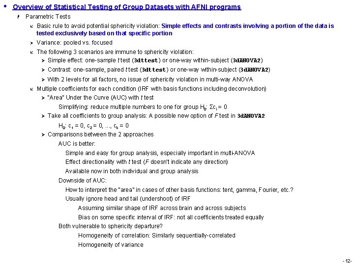
• Overview of Statistical Testing of Group Datasets with AFNI programs H Parametric Tests å Basic rule to avoid potential sphericity violation: Simple effects and contrasts involving a portion of the data is tested exclusively based on that specific portion Ø Variance: pooled vs. focused å The following 3 scenarios are immune to sphericity violation: Ø Simple effect: one-sample t test (3 dttest) or one-way within-subject (3 d. ANOVA 2) Ø Contrast: one-sample, paired t test (3 dttest) or one-way within-subject (3 d. ANOVA 2) Ø With 2 levels for all factors, no issue of sphericity violation in multi-way ANOVA å Multiple coefficients for each condition (IRF with basis functions including deconvolution) Ø “Area” Under the Curve (AUC) with t test Simplifying: reduce multiple numbers to one for group H 0: Σci = 0 Ø Take all coefficients to group analysis: A possible new option of F test in 3 d. ANOVA 2 H 0: c 1 = 0, c 2 = 0, . . . , c k = 0 Ø Comparisons between the 2 approaches AUC is better: Simple and easy for group analysis, especially important in multi-ANOVA Effect directionality with t test (F doesn’t indicate any direction) Available now in both individual and group analysis Downside of AUC: How to interpret the “area” in cases of other basis functions: tent, gamma, Fourier, etc. ? Usually ignore head and tail (undershoot) of IRF Assuming similar shape of IRF across brain and across subjects Bias on some specific interval of IRF: not all coefficients treated equally Both vulnerable to sphericity departure? Homogeneity of correlation: Similarly sequentially-correlated Homogeneity of variance -12 -

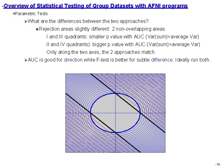
• Overview of Statistical Testing of Group Datasets with AFNI programs HParametric Tests ØWhat are the differences between the two approaches? v. Rejection areas slightly different: 2 non-overlapping areas I and III quadrants: smaller p value with AUC (Var(sum)>average Var) II and IV quadrants): bigger p value with AUC (Var(sum)>average Var) Only along the two axes, the 2 approaches match ØAUC is good for direction while F-test is better for subtle difference. Ideally run both. -13 -

• t-Test: 3 dttest H Student’s t distribution, developed by Gossett, tests if the mean of a set of data is different from a constant (usually 0) or the mean of another set of data. H 3 usages: one-sample, two-sample, and paired t test. H Assumptions H å Values in each set are normally distributed with equal variance å Sphericity issue? No issue of sphericity violation å Values in each set are independent? Compare a task between 2 groups: unpaired t-test å Values in each set are dependent? Compare two tasks for one group: paired t-test Example: effects of 2 conditions A and B at group level å Case 1: 15 subjects were given condition A v One-sample t test: effect of A is significant at group level μA = 0? å Case 2: 15 subjects under condition A and 13 other subjects under B v Two-sample t test: μA = μB (average response is the same? ) v OK with unequal sample sizes v Equivalent to 1 -way between-subject ANOVA å Case 3: 15 subjects under both conditions v Paired t test is used to test: μA = μB? v Equivalent to one-way within-subject (3 d. ANOVA 2 -type 3) v Equivalent to run one-sample t test on individual differences/contrasts -14 -

• t-Test: 3 dttest H Example: 2 -way (2 X 2) within-subject design (16 subjects) - AXBXC Ø 4 tasks (word, picture, spoken, sound) categorized as the following: Modality: visual, auditory Format: verbal, nonverbal visual verbal = word, visual nonverbal = picture, auditory verbal = spoken, auditory nonverbal = sound Ø What is the word or word-picture effect at group level? H 0: word = 0, or H 0: word-picture = 0 (one-sample t test!) Ø 3 d. ANOVA 3 -type 4 would not work because of lack of 2 nd contrast testing option Ø Can also run Group. Ana Ø Script of paired t test for H 0: word-picture = 0 3 dttest -prefix Wd-Pic Name of output dataset -paired We want a paired t test -set 1 Wd_S 1+tlrc. . . Wd_S 16+tlrc Input of first datasets -set 2 Pic_S 1+tlrc. . . Pic_S 16+tlrc Input of second datasets Ø Can also run a one-sample t test for H 0: word-picture = 0 Ø Picture/spoken/sound/ or spoken-sound/word-spoken/picture-sound effect? (quiz!) -15 -

• 1 -Way ANOVA: 3 d. ANOVA H H H Generalization of two-sample t-test å One-way between-subject å Null hypothesis H 0: no difference across all the factor levels (groups) å Examples of factor: subject group such as gender, age group, genotype, disease, etc. å OK with unequal sample sizes Assumptions å Values are normally distributed with equal variances across levels (groups) å Unlike regression analysis, no assumptions about relationship between dependent and independent variables (e. g. , not necessarily linear) å Independent variable (e. g. , gender, disease, genotype, etc. ) is qualitative 3 d. ANOVA versus 3 dttest å Equivalent when there are only two levels å More than 2 levels v Can still run two-sample t-test on paired levels with 3 dttest to obtain contrasts v Results should be similar unless there is significant heteroscedasticity across levels v Pooled variance vs. between-levels variance å 3 dttest is better if heteroscedasticity is significant across groups -16 -

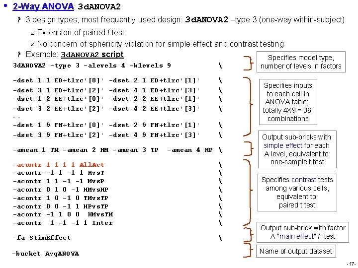
• 2 -Way ANOVA: 3 d. ANOVA 2 H 3 design types, most frequently used design: 3 d. ANOVA 2 –type 3 (one-way within-subject) Extension of paired t test å No concern of sphericity violation for simple effect and contrast testing Example: 3 d. ANOVA 2 script Specifies model type, å H 3 d. ANOVA 2 -type 3 -alevels 4 -blevels 9 -dset ED+tlrc'[1]' ED+tlrc'[3]' EE+tlrc'[1]' EE+tlrc'[3]' -dset 1 9 FN+tlrc'[0]' -dset 2 9 FN+tlrc'[1]' -dset 3 9 FN+tlrc'[2]' -dset 4 9 FN+tlrc'[3]' 1 3 1 1 2 2 ED+tlrc'[0]' ED+tlrc'[2]' EE+tlrc'[0]' EE+tlrc'[2]' -dset 2 4 1 1 2 2 … … -amean 1 TM -amean 2 HM -amean 3 TP -acontr -acontr 1 1 All. Act -1 1 Hvs. T 1 1 -1 -1 Mvs. P 0 1 0 -1 HMvs. HP 1 0 -1 0 TMvs. TP 0 0 -1 1 HPvs. TP -1 1 0 0 HMvs. TM 1 -1 -1 1 Inter -fa Stim. Effect -bucket Avg. ANOVA -amean 4 HP number of levels in factors Specifies inputs to each cell in ANOVA table: totally 4 X 9 = 36 combinations Output sub-bricks with simple effect for each A level, equivalent to one-sample t test Specifies contrast tests among various cells, equivalent to paired t test Output sub-brick with factor A “main effect” F test Name of output dataset -17 -

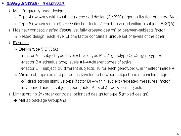
• 3 -Way ANOVA: 3 d. ANOVA 3 H Most frequently used designs å Type 4 (two-way within-subject) - crossed design (AXBXC): generalization of paired t-test å H Has new concept: nested design (vs. fully crossed design) or between-subjects factor å H Type 5 (two-way mixed) - classification factor A can’t be varied within a subject: BXC(A) Nested design: each level of one factor contains a unique set of levels of the other Example å Design type 5 BXC(A) v factor A = subject type; level #1=wild type P, #2=genotype Q, #3=genotype R v factor B = stimulus type; levels #1– 4=different types of tasks v factor C = subject; 30 different subjects, 10 for each genotype; C is “nested” inside A å Mixture of unpaired and paired tests with one between-subject and one within-subject v Paired across stimulus type (factor B) – within-subject (repeated-measures) factor v Unpaired across subject types (factor A levels) - between-subjects H Limitation: no 2 nd-order contrasts; balanced design for type 5 (mixed design) Matlab package Group. Ana -18 -

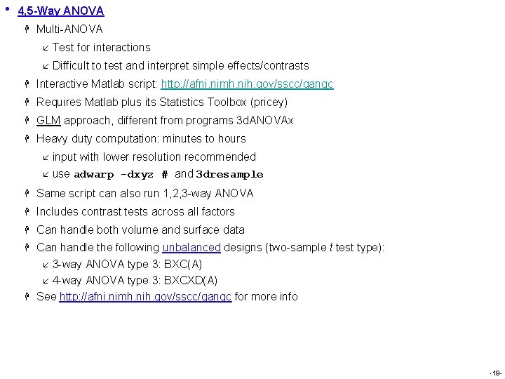
• 4, 5 -Way ANOVA H Multi-ANOVA å Test for interactions å Difficult to test and interpret simple effects/contrasts H Interactive Matlab script: http: //afni. nimh. nih. gov/sscc/gangc H Requires Matlab plus its Statistics Toolbox (pricey) H GLM approach, different from programs 3 d. ANOVAx H Heavy duty computation: minutes to hours å input with lower resolution recommended å use adwarp -dxyz # and 3 dresample H Same script can also run 1, 2, 3 -way ANOVA H Includes contrast tests across all factors H Can handle both volume and surface data H Can handle the following unbalanced designs (two-sample t test type): å 3 -way ANOVA type 3: BXC(A) å 4 -way ANOVA type 3: BXCXD(A) See http: //afni. nimh. nih. gov/sscc/gangc for more info H -19 -

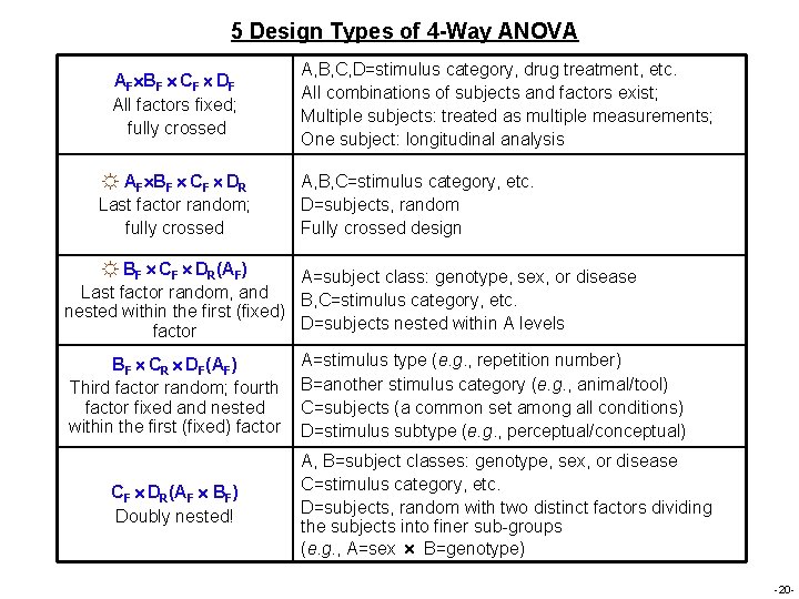
5 Design Types of 4 -Way ANOVA AF BF CF DF All factors fixed; fully crossed ☼ AF BF CF DR Last factor random; fully crossed A, B, C, D=stimulus category, drug treatment, etc. All combinations of subjects and factors exist; Multiple subjects: treated as multiple measurements; One subject: longitudinal analysis A, B, C=stimulus category, etc. D=subjects, random Fully crossed design ☼ BF CF DR(AF) A=subject class: genotype, sex, or disease Last factor random, and B, C=stimulus category, etc. nested within the first (fixed) D=subjects nested within A levels factor BF CR DF(AF) Third factor random; fourth factor fixed and nested within the first (fixed) factor CF DR(AF BF) Doubly nested! A=stimulus type (e. g. , repetition number) B=another stimulus category (e. g. , animal/tool) C=subjects (a common set among all conditions) D=stimulus subtype (e. g. , perceptual/conceptual) A, B=subject classes: genotype, sex, or disease C=stimulus category, etc. D=subjects, random with two distinct factors dividing the subjects into finer sub-groups (e. g. , A=sex B=genotype) -20 -

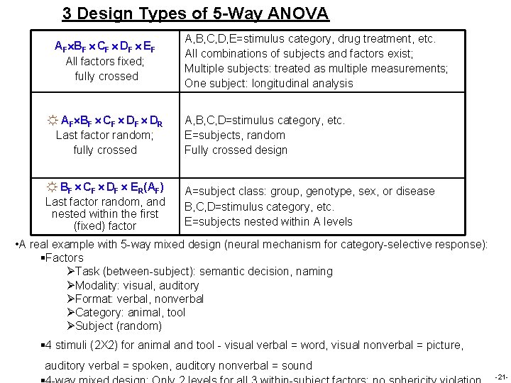
3 Design Types of 5 -Way ANOVA AF BF CF DF EF All factors fixed; fully crossed A, B, C, D, E=stimulus category, drug treatment, etc. All combinations of subjects and factors exist; Multiple subjects: treated as multiple measurements; One subject: longitudinal analysis ☼ AF BF CF DR Last factor random; fully crossed A, B, C, D=stimulus category, etc. E=subjects, random Fully crossed design ☼ BF CF DF ER(AF) Last factor random, and nested within the first (fixed) factor A=subject class: group, genotype, sex, or disease B, C, D=stimulus category, etc. E=subjects nested within A levels • A real example with 5 -way mixed design (neural mechanism for category-selective response): §Factors ØTask (between-subject): semantic decision, naming ØModality: visual, auditory ØFormat: verbal, nonverbal ØCategory: animal, tool ØSubject (random) § 4 stimuli (2 X 2) for animal and tool - visual verbal = word, visual nonverbal = picture, auditory verbal = spoken, auditory nonverbal = sound -21 -

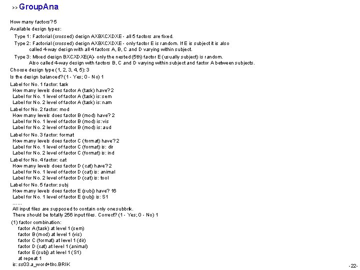
>> Group. Ana How many factors? 5 Available design types: Type 1: Factorial (crossed) design AXBXCXDXE - all 5 factors are fixed. Type 2: Factorial (crossed) design AXBXCXDXE - only factor E is random. If E is subject it is also called 4 -way design with all 4 factors A, B, C and D varying within subject. Type 3: Mixed design BXCXDXE(A)- only the nested (5 th) factor E (usually subject) is random. Also called 4 -way design with factors B, C and D varying within subject and factor A between subjects. Choose design type (1, 2, 3, 4, 5): 3 Is the design balanced? (1 - Yes; 0 - No) 1 Label for No. 1 factor: task How many levels does factor A (task) have? 2 Label for No. 1 level of factor A (task) is: sem Label for No. 2 level of factor A (task) is: nam Label for No. 2 factor: mod How many levels does factor B (mod) have? 2 Label for No. 1 level of factor B (mod) is: vis Label for No. 2 level of factor B (mod) is: aud Label for No. 3 factor: format How many levels does factor C (format) have? 2 Label for No. 1 level of factor C (format) is: dir Label for No. 2 level of factor C (format) is: ind Label for No. 4 factor: cat How many levels does factor D (cat) have? 2 Label for No. 1 level of factor D (cat) is: animal Label for No. 2 level of factor D (cat) is: tool Label for No. 5 factor: subj How many levels does factor E (subj) have? 16 Label for No. 1 level of factor E (subj) is: S 1 …… All input files are supposed to contain only one subbrik. There should be totally 256 input files. Correct? (1 - Yes; 0 - No) 1 (1) factor combination: factor A (task) at level 1 (sem) factor B (mod) at level 1 (vis) factor C (format) at level 1 (dir) factor D (cat) at level 1 (animal) factor E (subj) at level 1 (S 1) at repeat 1 is: ss 03. a_word+tlrc. BRIK -22 -

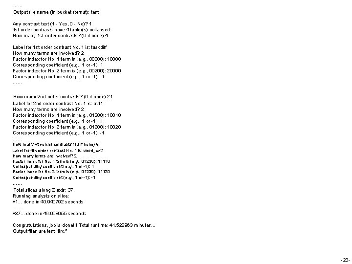
…… Output file name (in bucket format): test Any contrast test (1 - Yes, 0 - No)? 1 1 st order contrasts have 4 factor(s) collapsed. How many 1 st-order contrasts? (0 if none) 4 Label for 1 st order contrast No. 1 is: taskdiff How many terms are involved? 2 Factor index for No. 1 term is (e. g. , 00200): 10000 Corresponding coefficient (e. g. , 1 or -1): 1 Factor index for No. 2 term is (e. g. , 00200): 20000 Corresponding coefficient (e. g. , 1 or -1): -1 …… How many 2 nd-order contrasts? (0 if none) 21 Label for 2 nd order contrast No. 1 is: avt 1 How many terms are involved? 2 Factor index for No. 1 term is (e. g. , 01200): 10010 Corresponding coefficient (e. g. , 1 or -1): 1 Factor index for No. 2 term is (e. g. , 01200): 10020 Corresponding coefficient (e. g. , 1 or -1): -1 …… How many 4 th-order contrasts? (0 if none) 9 Label for 4 th order contrast No. 1 is: word_avt 1 How many terms are involved? 2 Factor index for No. 1 term is (e. g. , 01230): 11110 Corresponding coefficient (e. g. , 1 or -1): 1 Factor index for No. 2 term is (e. g. , 01230): 11120 Corresponding coefficient (e. g. , 1 or -1): -1 …… Total slices along Z axis: 37. Running analysis on slice: #1. . . done in 40. 940792 seconds …… #37. . . done in 49. 008655 seconds Congratulations, job is done!!! Total runtime: 41. 528963 minutes. . . Output files are test+tlrc. * -23 -

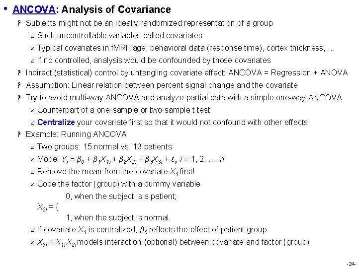
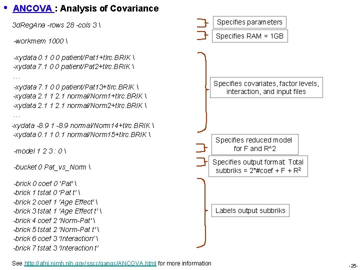
• ANCOVA: Analysis of Covariance H Subjects might not be an ideally randomized representation of a group å Such uncontrollable variables called covariates å Typical covariates in f. MRI: age, behavioral data (response time), cortex thickness, … å If no controlled, analysis would be confounded by those covariates H Indirect (statistical) control by untangling covariate effect: ANCOVA = Regression + ANOVA H Assumption: Linear relation between percent signal change and the covariate H Try to avoid multi-way ANCOVA and analyze partial data with a simple one-way ANCOVA H å Counterpart of a one-sample or two-sample t test å Centralize your covariate first so that it would not confound with other effects Example: Running ANCOVA å Two groups: 15 normal vs. 13 patients å Model Yi = β 0 + β 1 X 1 i + β 2 X 2 i + β 3 X 3 i + εi, i = 1, 2, . . . , n å Remove the mean from the covariate X 1 first! å Code the factor (group) with a dummy variable 0, when the subject is a patient; X 2 i = { 1, when the subject is normal. å If covariate X 1 is centralized, β 0 reflects the effect of patient group å X 3 i = X 1 i X 2 i models interaction (optional) between covariate and factor (group) -24 -

• ANCOVA : Analysis of Covariance 3 d. Reg. Ana -rows 28 -cols 3 -workmem 1000 -xydata 0. 1 0 0 patient/Pat 1+tlrc. BRIK -xydata 7. 1 0 0 patient/Pat 2+tlrc. BRIK … -xydata 7. 1 0 0 patient/Pat 13+tlrc. BRIK -xydata 2. 1 1 2. 1 normal/Norm 1+tlrc. BRIK -xydata 2. 1 1 2. 1 normal/Norm 2+tlrc. BRIK … -xydata -8. 9 1 -8. 9 normal/Norm 14+tlrc. BRIK -xydata 0. 1 1 0. 1 normal/Norm 15+tlrc. BRIK -model 1 2 3 : 0 -bucket 0 Pat_vs_Norm -brick 0 coef 0 ‘Pat’ -brick 1 tstat 0 ‘Pat t' -brick 2 coef 1 'Age Effect' -brick 3 tstat 1 'Age Effect t' -brick 4 coef 2 'Norm-Pat' -brick 5 tstat 2 'Norm-Pat t' -brick 6 coef 3 'Interaction' -brick 7 tstat 3 'Interaction t' See http: //afni. nimh. nih. gov/sscc/gangc/ANCOVA. html for more information Specifies parameters Specifies RAM = 1 GB Specifies covariates, factor levels, interaction, and input files Specifies reduced model for F and R^2 Specifies output format: Total subbriks = 2*#coef + F + R 2 Labels output subbriks -25 -

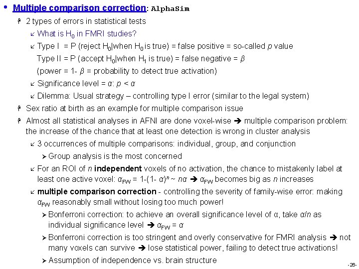
• Multiple comparison correction: Alpha. Sim H 2 types of errors in statistical tests å What is H 0 in FMRI studies? å Type I = P (reject H 0|when H 0 is true) = false positive = so-called p value Type II = P (accept H 0|when H 1 is true) = false negative = β (power = 1 - β = probability to detect true activation) å Significance level = α: p < α å Dilemma: Usual strategy – controlling type I error (similar to the legal system) H Sex ratio at birth as an example for multiple comparison issue H Almost all statistical analyses in AFNI are done voxel-wise multiple comparison problem: the increase of the chance that at least one detection is wrong in cluster analysis å 3 occurrences of multiple comparisons: individual, group, and conjunction Ø Group analysis is the most concerned å For an ROI of n independent voxels of no activation, the chance to mistakenly label at least one active voxel: αFW = 1 -(1 - α)n ~ nα αFW becomes big as n increases å multiple comparison correction - controlling the severity of family-wise error: making αFW reasonably small without losing too much power! Ø Bonferroni correction: to achieve an overall significance level of α, take α/n as individual significance level αFW = α Ø Bonferroni correction is too stringent and overly conservative for FMRI analysis not many voxels can survive lose statistical power, failing to detect true activations! Ø Assumption of independence vs. brain structure -26 -

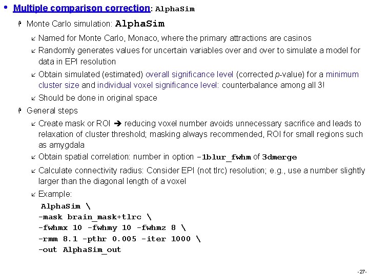
• Multiple comparison correction: Alpha. Sim H H Monte Carlo simulation: Alpha. Sim å Named for Monte Carlo, Monaco, where the primary attractions are casinos å Randomly generates values for uncertain variables over and over to simulate a model for data in EPI resolution å Obtain simulated (estimated) overall significance level (corrected p-value) for a minimum cluster size and individual voxel significance level: counterbalance among all 3! å Should be done in original space General steps Create mask or ROI reducing voxel number avoids unnecessary sacrifice and leads to relaxation of cluster threshold; masking always recommended, ROI for small regions such as amygdala å Obtain spatial correlation: number in option -1 blur_fwhm of 3 dmerge å å Calculate connectivity radius: Consider EPI (not tlrc) resolution; e. g. , use a number slightly larger than the diagonal length of a voxel å Example: Alpha. Sim -mask brain_mask+tlrc -fwhmx 10 -fwhmy 10 -fwhmz 8 -rmm 8. 1 -pthr 0. 005 -iter 1000 -out Alpha. Sim_out -27 -

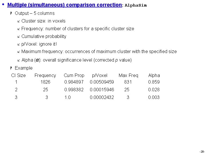
• Multiple (simultaneous) comparison correction: Alpha. Sim H H Output – 5 columns å Cluster size: in voxels å Frequency: number of clusters for a specific cluster size å Cumulative probability å p/Voxel: ignore it! å Maximum frequency: occurrences of maximum cluster with the specified size å Alpha (α): overall significance level (corrected p value) Example Cl Size Frequency Cum Prop p/Voxel Max Freq Alpha 1 1826 0. 984897 0. 00509459 831 0. 859 2 25 0. 998382 0. 00015946 25 0. 028 3 1. 0 0. 00002432 3 0. 003 -28 -

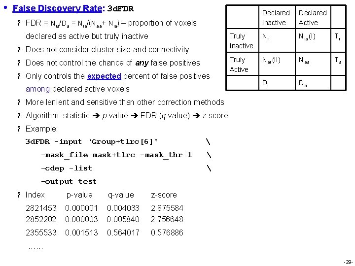
• False Discovery Rate: 3 d. FDR H Declared Inactive Declared Active Truly Inactive Nii Nia (I) Ti Truly Active Nai (II) Naa Ta Di Da FDR = Nia/Da = Nia/(Naa+ Nia) – proportion of voxels declared as active but truly inactive H Does not consider cluster size and connectivity H Does not control the chance of any false positives H Only controls the expected percent of false positives among declared active voxels H More lenient and sensitive than other correction methods H Algorithm: statistic p value FDR (q value) z score H Example: 3 d. FDR -input ‘Group+tlrc[6]' -mask_file mask+tlrc -mask_thr 1 -cdep -list -output test H Index p-value q-value z-score 2821453 0. 000001 0. 004033 2. 875584 2852202 0. 000003 0. 005840 2. 756648 2355533 0. 001513 0. 564017 0. 576886 …… -29 -

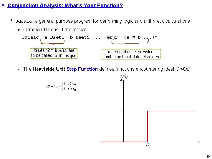
• Conjunction Analysis: What’s Your Function? H 3 dcalc: a general purpose program for performing logic and arithmetic calculations å Command line is of the format 3 dcalc -a Dset 1 -b Dset 2. . . -expr “(a * b. . . )” values from Dset 1 are to be called ‘a’ in -expr å mathematical expression combining input dataset values The Heaviside Unit Step Function defines functions encountering ideal On/Off: -30 -

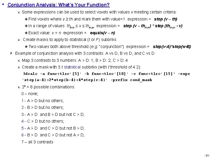
• Conjunction Analysis: What’s Your Function? å Some expressions can be used to select voxels with values v meeting certain criteria: v Find voxels where v th and mark them with value=1 expression = step (v – th) v In a range of values: thmin ≤ v ≤ thmax expression = step (v – thmin) * step (thmax - v) v Exact value: v = n expression = equals(v – n) å Create masks to apply to statistical (t or F) subbriks v Two values both above threshold (e. g. “conjunction”) expression = step(v-A)*step(w-B) H Example of conjunction analysis with 3 contrasts: A vs D, B vs D, and C vs D å Map 3 contrasts to 3 numbers: A > D: 1; B > D: 2; C > D: 4 å Create a mask with 3 t statistical subbriks (with t threshold of 4. 2): 3 dcalc -a func+tlrc'[5]' -b func+tlrc'[10]' -c func+tlrc'[15]‘ -expr 'step(a-4)+2*step(b-4)+4*step(c-4)' -prefix cond_mask å 23 = 8 possible combinations: 0 – none; 1 - A > D but no others; 2 - B > D but no others; 3 - A > D and B > D but not C > D; 4 - C > D but no others; 5 - A > D and C > D but not B > D; 6 - B > D and C > D but not A > D; 7 – all 3 contrasts -31 -