Introduction Knowledge Engineering Ronald Westra Eric Postma Department

Introduction Knowledge Engineering Ronald Westra, Eric Postma Department of Mathematics Universiteit Maastricht

Introduction Knowledge Engineering Lecture 3 Modelling of Dynamical Systems

Introduction Knowledge Engineering How to survive this course…

Introduction Knowledge Engineering

Introduction Knowledge Engineering How to find this lecture … http: //www. math. unimaas. nl/personal/ronaldw/E ducation/IKT_page. htm

Introduction Knowledge Engineering 3. 1 On Growth and Decay

Growth and Decay • Examples of Growth and Decay – Unlimited growth – Limited growth • Modelling growth and decay in nature – Exponential decay of foraging paths – Growth of knowledge –…

Growth and decay • Growth and decay: two sides of the same coin • Growth – At each step: replace each element by n elements • Decay – At each step: replace n elements by one element

Mathematical description • Mathematicians like to make short statements • Instead of saying: – At time t seconds the quantity is n times the quantity at t-1 seconds • They say: – P(t) = n P(t-1)

plot for P(t) = n. P(t-1) P(t) t

Logarithms • The rapid growth makes it hard to draw • Trick: express quantities in terms of their number of zeros • A logarithmic plot of P(t) = n P(t-1) makes the curves straight…

Logarithmic plot for P(t) = n. P(t-1) Log(P(t)) t

From growth to decay • We can perform the same trick with decay • Instead of saying: – At time t seconds the quantity is 1/n times the quantity at t-1 seconds • Mathematicians say: – P(t) = (1/n) P(t-1)

plot for P(t) = (1/n)P(t-1) P(t) t

Logarithmic plot for P(t) = (1/n)P(t-1) Log(P(t)) t

Introduction Knowledge Engineering EXAMPLE: Growth of Bacterial Populations

Growth of a population of bacteria • Consider a controlled laboratory environment: • Bacteria are single cell micro organisms which reproduce by cell division. • They live from nutrition provided in the laboratory setting • There is plenty of space to multiply

Modelling population growth • Each cell divides after a constant amount of time. • Initially cells are of different, unrelated, ages • During a period of time Δ, the amount of cells which split is proportional to the size of the population.

Modelling population growth • The rate of change is proportional to the population size: • Let N(t) be a function specifying the number of cells at time t, t ≥ 0. • Then it must hold that • Differential equation: N’ = β N. • (where N’ is the first order derivative of N ).

Which function N satisfies the equation? • Could N be a polynomial? • N(t)= ao + a 1 t + a 2 t 2 + …. + an tn. N’(t) = a 1 + a 2 t + a 3 t 2 + …. + an tn-1. N(t’) ≠ N(t) • N cannot be a polynomial!

Which function N satisfies the equation? • Can N be an exponential function? • N(t) = αeγt N’(t) = γαeγt N’(t) = γ N(t) as required.

What is the value of α? • Let no be the initial population size, that is, N(0) = no. • Then no = N(0) = αeγ 0 = α.

Definitions • N’ = β N is called a linear homogenous first order differential equation, because 1. It is a linear function, 2. it involves only the first order derivative, 3. it only considers the function and its derivative.

Conclusion • The linear first order homogenous difference equation • xn+1 = a xn • has solution xn = an xo. • This problem can be solved without ‘algorithm’, the analytical solution is a formula. • Notice that xn converges, reaches an equilibrium if and only if |a| < 1.

Introduction Knowledge Engineering 3. 2 Bounded Growth

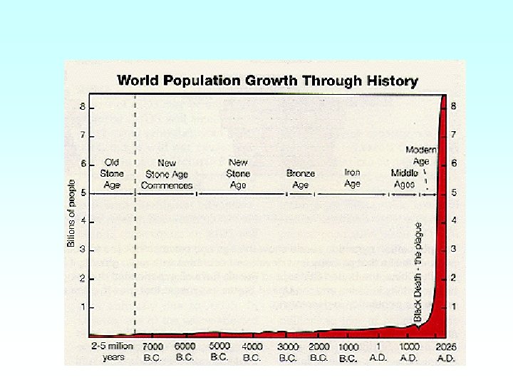
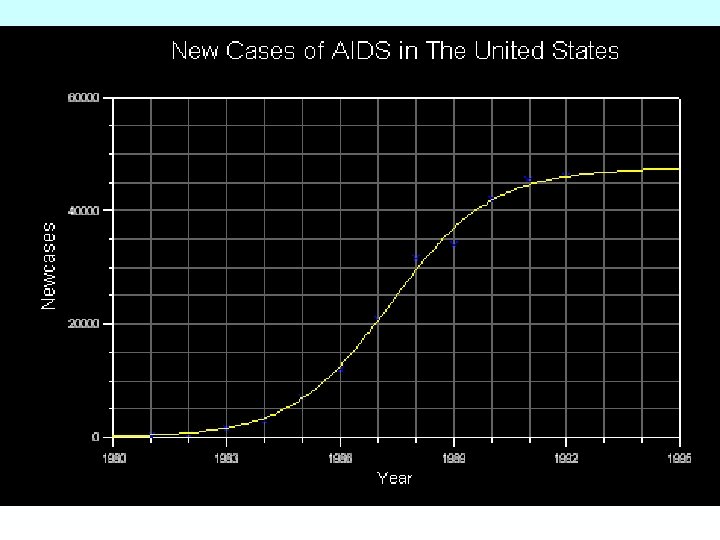
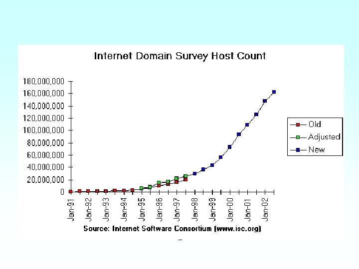
Unlimited growth P(t) = n. P(t-1) • In most cases, there is a limit to the growth • Although this is obvious, it is often forgotten, e. g. , – – – World population growth Spreading of disease (AIDS) Internet hype Success …

Bounded growth • Apparently, growth is generally bounded • An S-shaped curve is characteristic for bounded growth • The logistic curve

Bounded growth (Verhulst) P(t+1) = n P(t) (1 -P(t)) Logistic model a. k. a. the Verhulst model • How do you state this model in a linguistic form? • Pn is the fraction of the maximum population size 1 • n is a parameter indicating time

Balancing growth and decay • The Verhulst model balances growth: P(t+1) = n P(t) • With decay P(t+1) = n (1 -P(t))

P(t+1) = 1. 5 P(t) (1 -P(t))

Problems with the logistic function as a model for population growth : Verhulst attempted to fit a logistic curve to 3 separate censuses of the population of the United States of America in order to predict future growth. All 3 sets of predictions failed. In 1924, Professor Ray Pearl and Lowell J. Reed used Verhulst's model to predict an upper limit of 2 billion for the world population. This was passed in 1930. A later attempt by Pearl and an associate Sophia Gould in 1936 then estimated an upper limit of 2. 6 billion. This was passed in 1955.

Bounded growth • Apparently, growth is generally bounded • An S-shaped curve is characteristic for bounded growth • The logistic curve (e. g. , the Verhulst equation)

Introduction Knowledge Engineering 3. 3 Predator-Prey Models

Recall the Logistic Model Large P slows down P Logistic model a. k. a. the Verhulst model • Pn is the fraction of the maximum population size 1 • is a parameter

Interacting quantities • The logistic model describes the dynamics (change) of a single quantity interacting with itself • We now move to models describing two (or more) interacting quantities

Fish statistics • Vito Volterra (1860 -1940): a famous Italian mathematician • Father of Humberto D'Ancona, a biologist studying the populations of various species of fish in the Adriatic Sea • The numbers of species sold on the fish markets of three ports: Fiume, Trieste, and Venice.

percentages of predator species (sharks, skates, rays, . . )

Volterra’s model • Two (simplifying) assumptions – The predator species is totally dependent on the prey species as its only food supply – The prey species has an unlimited food supply and no threat to its growth other than the specific predator prey

Two Populations P and Q xt is the prey-population yt is the predator-population a, b, c, d are parameters

Behaviour of the Volterra’s model Oscillatory behaviour Limit cycle

Effect of changing the parameters (1) Behaviour is qualitatively the same. Only the amplitude changes.

Effect of changing the parameters (2) Behaviour is qualitatively different. A fixed point instead of a limit cycle.

Why are PP models useful? • They model the simplest interaction among two systems and describe natural patterns • Repetitive growth-decay patterns, e. g. , – World population growth – Diseases –… Exponential growth Limited growth Exponential decay Oscillation time

Introduction Knowledge Engineering 3. 4 Fibonacci

Fibonacci’s rabbits • Around the year 1200, the italian mathematician Fibonacci asked himself the following question. • I start with a single newborn rabbit-pair. Mature rabbit pairs create offspring every month. Rabbit pairs are mature from the second month. How many rabbits do I have after t months? (assuming rabbits live forever)

A second order differential equation • Let Kn be the number of rabbits after n month. Then it must hold that • Kn = Kn-1 + Kn-2. Linear homegenous second order difference equation • Because all pairs of rabbits that lived in Kn-1 are still alive in Kn, and all pairs that were alive in Kn-2 produced a pair of offspring.

Solving the 2 nd order difference equation • Kn - Kn-1 - Kn-2 = 0. • Let’s guess a solution once again… • K n = k λ n. • Then it must hold that • k λn+2 - k λn+1 - k λn = 0. • k λn (λ 2 - λ - 1 ) = 0.

Solving the 2 nd order difference equation • There are two solutions: 1. λn = 0 for all n = 1, 2, …. 2. but we didn’t start with zero rabbits… 2. (λ 2 - λ - 1) = 0. • [1 +/- √ (1 - 4*1*-1)]/2 • = [½ +/- ½ √ 5 ].

Solving the 2 nd order difference equation • Thus there are 2 solutions: • λ 1 = ½ + ½ √ 5 and λ 2 = ½ - ½ √ 5. • The differential equation • Kn - Kn-1 - Kn-2 has solution • Kn = k 1 * (½ + ½ √ 5)n + k 2 * (½ - ½ √ 5)n

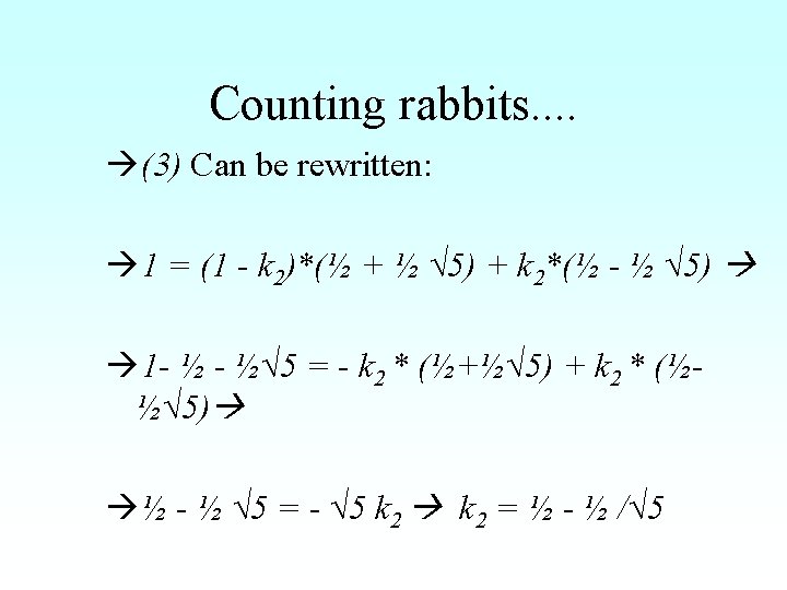
Fibonacci’s starting conditions • Fibonacci started with newborn rabbits, thus K 0 = 1, K 1=1. 1= k 1*(½ + ½ √ 5)0 + k 2*(½ - ½ √ 5)0 (1) • 1 = k 1*(½ + ½ √ 5)1 + k 2*(½ - ½ √ 5)1 (2) (1) can be rewritten to k 1= 1 - k 2

Fibonacci’s starting conditions • From (2) • 1 = k 1*(½ + ½ √ 5)1 + k 2*(½ - ½ √ 5)1 • and the rewritten (1) • k 1=1 - k 2 • it follows that • 1 = (1 - k 2)*(½ + ½ √ 5) + k 2*(½ - ½ √ 5) (3)

Still counting rabbits. . . • • From k 2 = ½ - ½ /√ 5 and k 1=1 - k 2 it follows that • k 1=1 – (½ - ½ /√ 5) = ½ + ½ /√ 5 • Thus the solution to the difference equation is • Kn = (½+½ /√ 5) * (½+½ √ 5)n + (½-½ /√ 5) * (½-½ √ 5)n

Introduction Knowledge Engineering 3. 5 The random walk model

Two examples from research • Modelling foraging – Decaying step-lengths in foraging • Modelling semantic network dynamics – Growth of knowledge

Foraging patterns in nature Random walk Levy flight

Distribution of step lengths l What is the slope of decay?

Slope of the log plot equals

Universal foraging behaviour • Foraging behaviour in sparse food environments is characterised by Lévy-flights with 2 is performed by: – – Albatrosses foraging bumblebees Deer Amoebas • In dense food environments > 3 (random walk)

Introduction Knowledge Engineering 3. 6 Small World Networks

Growth of knowledge semantic networks lemon gravitation pear apple Newton orange • Average separation should be small • Local clustering should be large Einstein

Semantic net at age 3

Semantic net at age 4

Semantic net at age 5

The growth of semantic networks obeys a logistic law

• Given the enormous size of our semantic networks, how do we associate two arbitrary concepts?

Clustering coefficient and Characteristic Path Length • Clustering Coefficient (C) – The fraction of associated neighbors of a concept • Characteristic Path Length (L) – The average number of associative links between a pair of concepts

Example lemon gravitation pear apple orange Newton Einstein

Four network types a c b d

Network Evaluation Type of network k C L Fully-connected N-1 Large Small Random <<N Small Regular <<N Large Small-world <<N Large Small

Varying the rewiring probability p: from regular to random networks 1 C(p)/C(0) L(p)/L(0) 0 0. 00001 0. 1 1. 0 p

Data set: two examples APPLE PIE PEAR ORANGE TREE CORE FRUIT (20) (17) (13) ( 8) ( 7) ( 4) NEWTON APPLE ISAAC LAW ABBOT PHYSICS SCIENCE (22) (15) ( 8) ( 6) ( 4) ( 3)

L as a function of age (× 100) = semantic network = random network

C as a function of age (× 100) = semantic network = random network

Small-worldliness Walsh (1999) • Measure of how well small path length is combined with large clustering • Small-wordliness = (C/L)/(Crand/Lrand)

Small-worldliness as a function of age adult

Small-Worldliness Some comparisons 5 4 3. 5 3 2. 5 2 1. 5 1 0. 5 0 Semantic Network Cerebral Cortex Caenorhabditis Elegans

What causes the smallworldliness in the semantic net? • TOP 40 of concepts • Ranked according to their k-value (number of associations with other concepts)

Semantic top 40

Introduction Knowledge Engineering 3. 7 Equilibria and Steady State

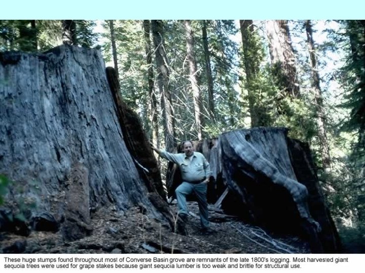
More complicated interactions • Clinton established the Giant Sequoia National Monument to protect the forest from culling, logging and clearing. – But many believe that Clinton’s measures added fuel to the fires. – Tree-thinning is required to prevent large fires. – Fires are required to clear land to promote new growth. • “Smokey Bear did too good a job, ” said Matt Mathes, a Forest Service spokesman. “It was a well-meaning policy with unintentional consequences. ”

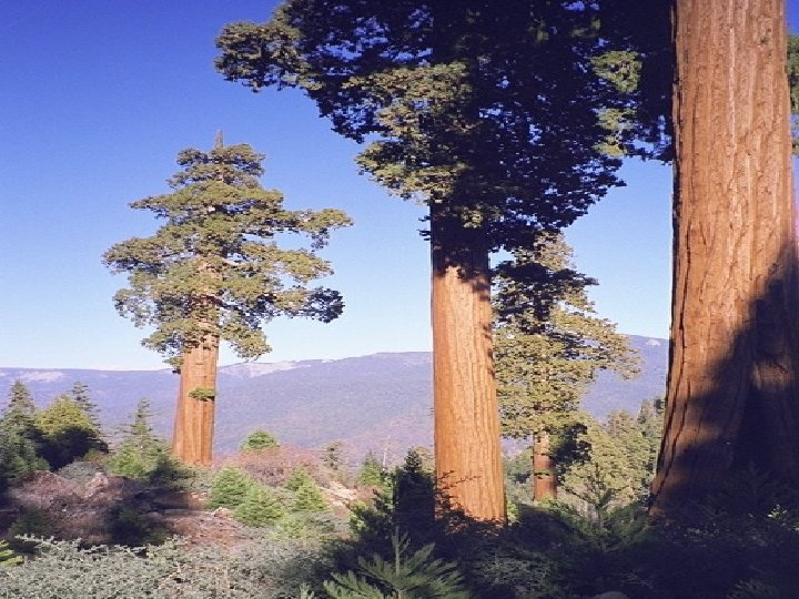
Sequoias

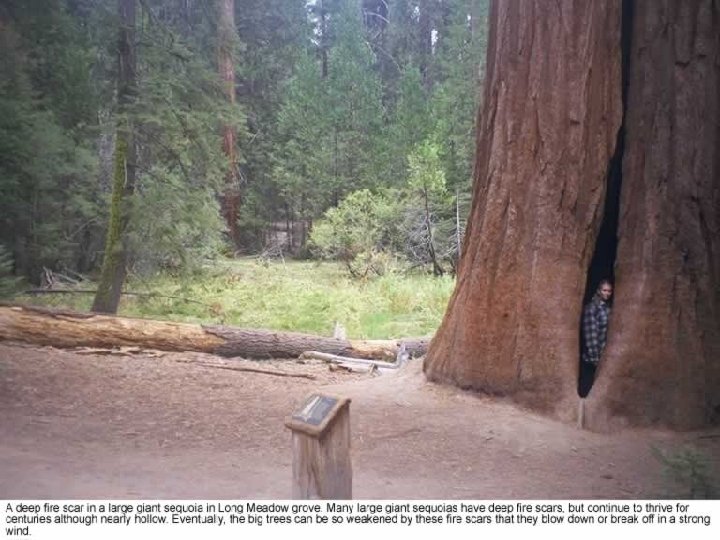
Predator versus Prey? Fire is dangerous when caused by surrounding bushes Fire is needed to clean area and to open the seeds of the Sequoia • Fire acts as “prey” because it is needed for growth • Fire acts as “predator” because it may set the tree on fire • Tree acts as “prey” for the predator • If trees die out, the predator dies out too

Predators, Preys and Hurricanes

Biodiversity “Human alteration of the global environment has triggered the sixth major extinction event in the history of life and caused widespread changes in the global distribution of organisms. These changes in biodiversity alter ecosystem processes and change the resilience of ecosystems to environmental change. This has profound consequences for services that humans derive from ecosystems. The large ecological and societal consequences of changing biodiversity should be minimized to preserve options for future solutions to global environmental problems. ” F. Stuart Chapin III et al. (2000)

The role of biodiversity in global change

Model predictions • Predicted relative change in biodiversity in 2100 – – – – T = Tropical forest G = Grasslands M = Mediterranean D = Dessert N = Northern forests B = Boreal forests A = Arctic

Consequences of reduced biodiversity ". . . decreasing biodiversity will tend to increase the overall mean interaction strength, on average, and thus increase the probability that ecosystems undergo destabilizing dynamics and collapses. " Kevin Shear Mc. Cann (2000)

“equilibrium” states • Complex systems are assumed to converge towards an equilibrium state. Equilibrium state: two (or more) opposite processes take place at equal rates VIDEO unstable

Over-predation and extinction

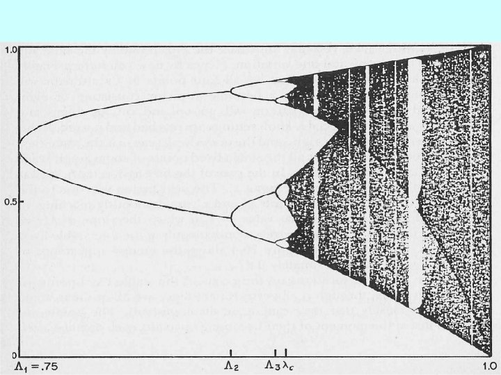
Introduction Knowledge Engineering 3. 8 Chaotic Systems

Deterministic versus Stochastic Models • Deterministic model – The state at time t+1 is fully determined by the state at time t • Stochastic model – The state at time t+1 is partially determined by the state at time t, and partially by noise

What is noise? • Noise is randomness • Noise is unpredictable – except for statistical descriptors such as mean, standard deviation, etc. • Example – A die generates random numbers ranging from 1 to 6 – At any time t the number generated by the die is unpredictable – The probability of a certain number occurring is predictable

What is determinism? • The Verhulst equation is an example of a deterministic model – The value at time n+1 is fully determined by the value at time n

Fundamental question • Given perfect knowledge about the positions and velocities of all particles in the universe, can we predict the future state of the universe? • Preliminary answers – YES if the universe is deterministic – NO if the universe is stochastic

Turbulence • “Chaotic” behaviour of many-particle systems • Was poorly understood until chaos theory emerged • Was known to arise from non-linear interactions

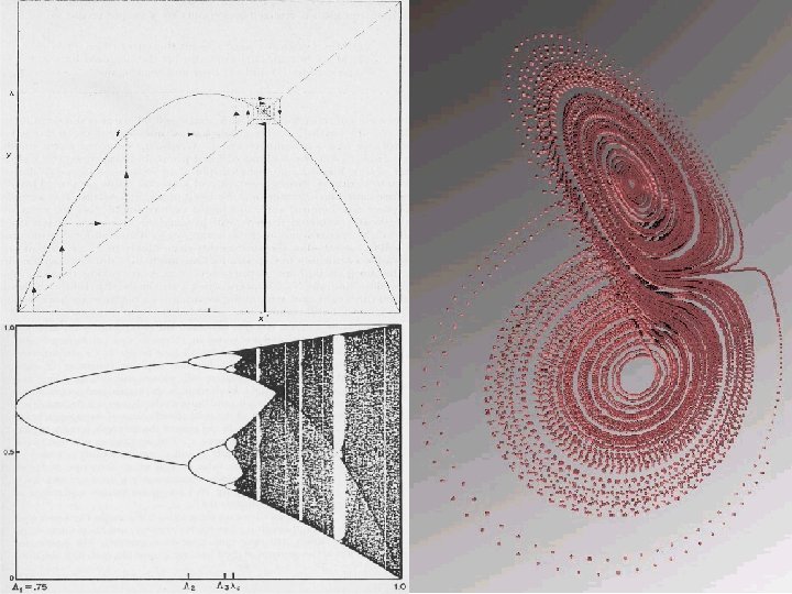
A “folded” function is needed

Graphical analysis ( =0. 7) y=f(x)=x(t+1) x(t)

Strange attractors • The state of chaotic systems does not converge onto a point or limit cycle but on a chaotic attractor • The same state never reoccurs because that would lead to periodicity • Very small deviations in starting conditions are amplified

Hénon attractor

• Self-similarity across scales • Fractals – Coastlines – Mountains – Etc.

Deterministic Chaos • Implication for deterministic models – Prediction of future states is limited by the sensitivity to initial conditions – Hence, despite determinism, future states cannot be predicted due to inevitable measurement errors – Measurement errors may be very small, but always larger than zero – Errors are amplified due to the chaotic trajectory • E. g. , Lorentz equations

Lorentz attractor

Fundamental question (reprise) • Given perfect knowledge about the positions and velocities of all particles in the universe, can we predict the future state of the universe? • Answers – NO if the universe is deterministic – NO if the universe is stochastic

Quote from Robert May (1976)

Predicting War • Collapse of nations, three factors 1. Infant mortality 2. Level of democracy 3. Openness to international trade • But is the course of history predictable? – Small changes can have large effects

Controlling Physiological Chaos • Nerve tissue: nonlinear coupled system • Congestive Heart Failure (CHF) • Chaos is good for you

Chaos and Chaotic Models in Neurosystems The Freeman-Skarda model of the Olfactory Bulb

The Freeman-Skarda model of the Olfactory Bulb

Conclusions • In this lecture, we have been modeling dynamic systems. • For the studied examples, we have always been able to model them using a linear equation, that we could solve analytically. • Hence no algorithms were required! • In general, there are many systems of differential equations for which analytical solutions are not known, and for which more algorithmic approaches are used to solve them.