Hyperspectral Remote Sensing Workshop Instructor Dr Ronald G

Hyperspectral Remote Sensing Workshop Instructor: Dr. Ronald G. Resmini rresmini@mitre. org and rresmini@gmu. edu ASPRS/Potomac Region’s Geo. Tech 2013 Keck Center, National Academies, Washington, DC 10 December 2013 1

Dr. Ronald G. Resmini The MITRE Corporation and George Mason University Please call me Ron v: 703 -470 -3022 rresmini@mitre. org and rresmini@gmu. edu http: //mason. gmu. edu/~rresmini/ 2

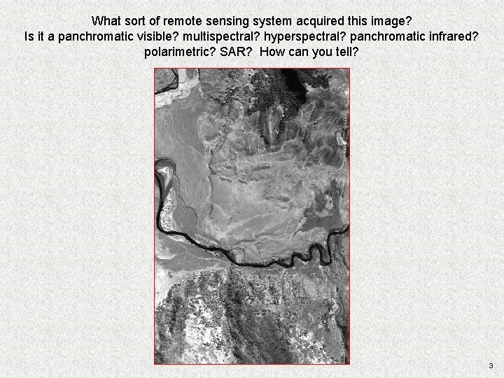
What sort of remote sensing system acquired this image? Is it a panchromatic visible? multispectral? hyperspectral? panchromatic infrared? polarimetric? SAR? How can you tell? 3

Introduction to Hyperspectral Imagery (HSI) Remote Sensing and to ENVI® 4

Introduction to Hyperspectral Imagery (HSI) Remote Sensing HSI is, fundamentally: writ large. . . the phenomenology of spectra; remote material detection, identification, characterization and quantification 5

HSI Remote Sensing: Frame of Reference. . . • Remote sensing of the earth Øairborne Øspaceborne Øground (portables) • But bear in mind other apps: Ømedical Øindustrial Ømany, many others 6

Applications of HSI RS • Geology • Forestry • Agriculture • Mapping/land use, land cover analysis • Atmospheric analysis • Environmental monitoring • Littoral zone RS • Many, many others 7

• Where/how do we do HSI remote sensing? • What is the nature of what is measured? • What is there to measure? • How is it done? • Are there distinguishing observables? • etc. . . 8

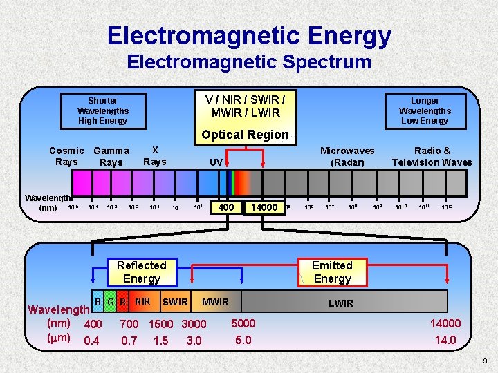
Electromagnetic Energy Electromagnetic Spectrum V / NIR / SWIR / Electromagnetic Spectrum Shorter Wavelengths High Energy Longer Wavelengths Low Energy MWIR / LWIR Optical Region Cosmic Gamma Rays Wavelength (nm) 10 -5 10 -4 10 -3 10 -2 X Rays 10 -1 Microwaves (Radar) UV 10 101 400 14000 105 106 Reflected Energy B G R NIR Wavelength (nm) 400 ( m) 0. 4 SWIR 107 108 109 Radio & Television Waves 1010 1011 1012 Emitted Energy MWIR 700 1500 3000 0. 7 1. 5 3. 0 LWIR 5000 5. 0 LWIR 14000 14. 0 9

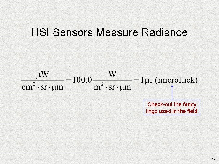
HSI Sensors Measure Radiance Check-out the fancy lingo used in the field 10

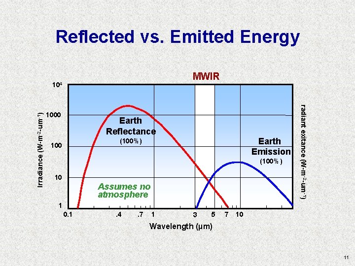
Reflected vs. Emitted Energy MWIR 1000 Earth Reflectance Earth Emission (100%) 100 (100%) 10 Assumes no atmosphere radiant exitance (W-m-2 -um-1) Irradiance (W-m-2 -um-1) 104 1 0. 1 . 4 . 7 1 3 5 7 10 Wavelength (µm) 11

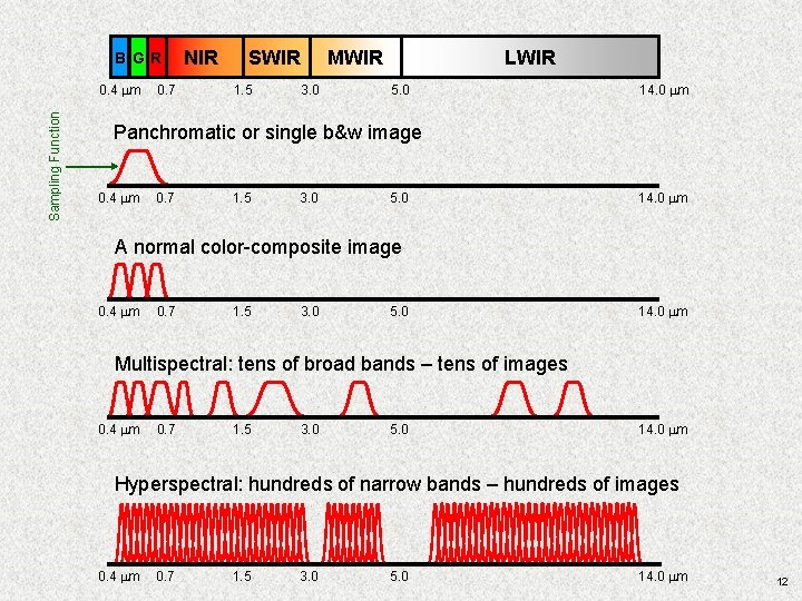
B GR Sampling Function 0. 4 mm 0. 7 NIR SWIR 1. 5 LWIR MWIR 3. 0 5. 0 14. 0 mm Panchromatic or single b&w image 0. 4 mm 0. 7 1. 5 3. 0 5. 0 14. 0 mm A normal color-composite image 0. 4 mm 0. 7 1. 5 3. 0 5. 0 14. 0 mm Multispectral: tens of broad bands – tens of images 0. 4 mm 0. 7 1. 5 3. 0 5. 0 14. 0 mm Hyperspectral: hundreds of narrow bands – hundreds of images 0. 4 mm 0. 7 1. 5 3. 0 5. 0 14. 0 mm 12

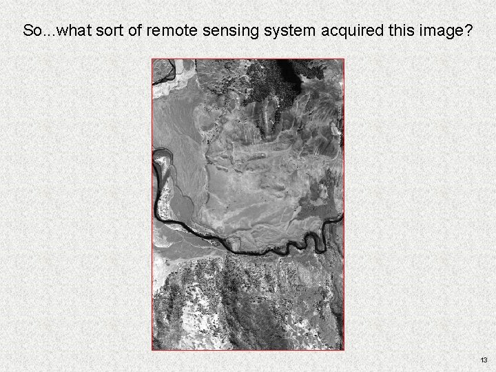
So. . . what sort of remote sensing system acquired this image? 13

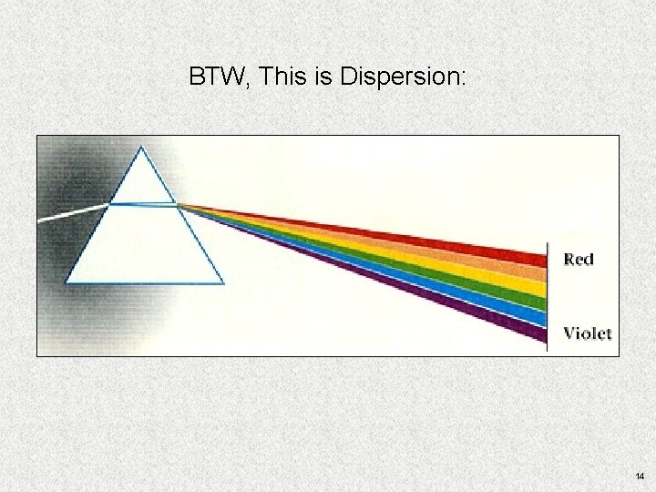
BTW, This is Dispersion: 14

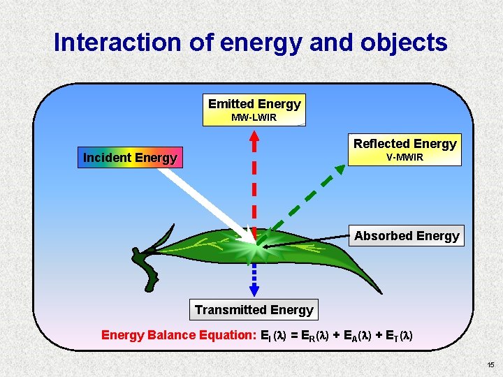
Interaction of energy and objects Emitted Energy MW-LWIR Reflected Energy Incident Energy V-MWIR Absorbed Energy Transmitted Energy Balance Equation: EI ( ) = ER( ) + EA( ) + ET( ) 15

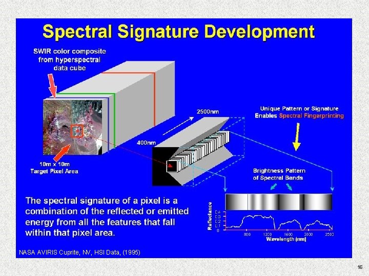
NASA AVIRIS Cuprite, NV, HSI Data, (1995) 16

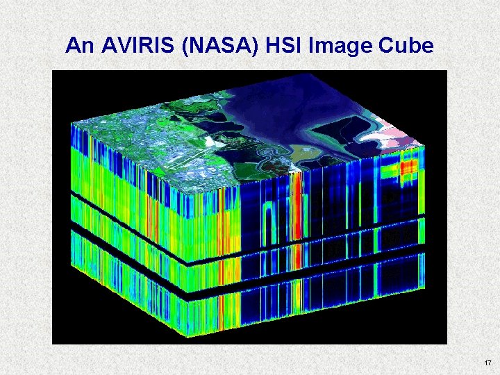
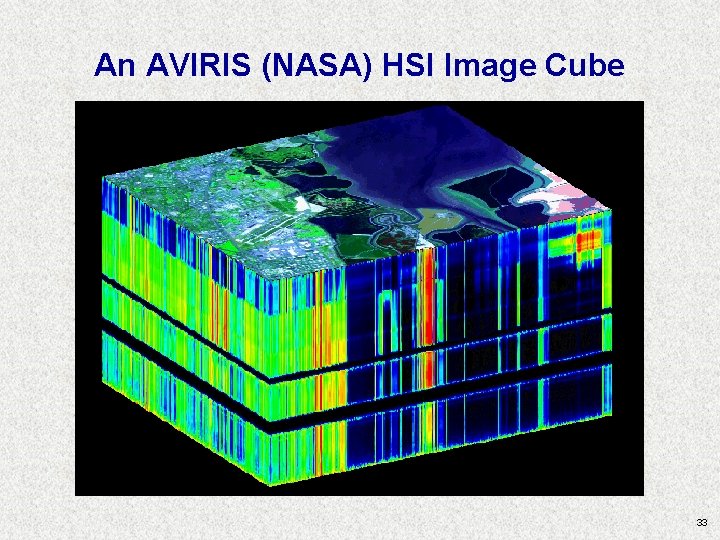
An AVIRIS (NASA) HSI Image Cube 17

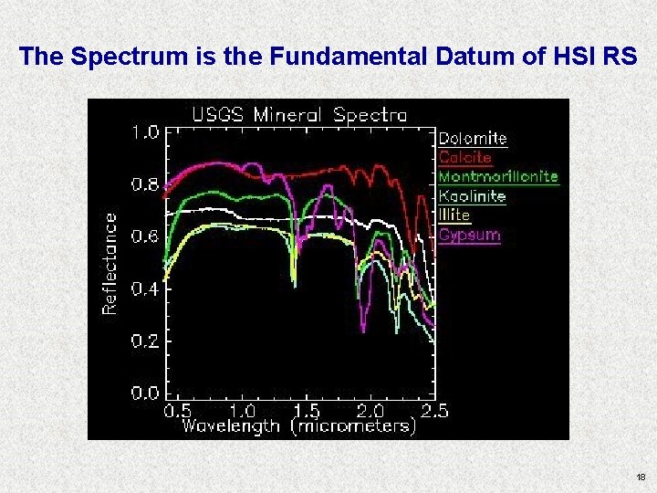
The Spectrum is the Fundamental Datum of HSI RS 18

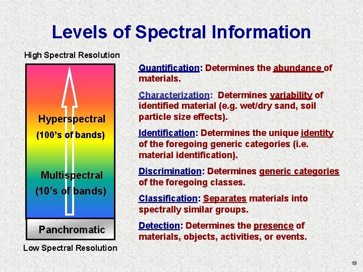
Levels of Spectral Information High Spectral Resolution Quantification: Determines the abundance of materials. Hyperspectral (100’s of bands) Multispectral (10’s of bands) Panchromatic Characterization: Determines variability of identified material (e. g. wet/dry sand, soil particle size effects). Identification: Determines the unique identity of the foregoing generic categories (i. e. material identification). Discrimination: Determines generic categories of the foregoing classes. Classification: Separates materials into spectrally similar groups. Detection: Determines the presence of materials, objects, activities, or events. Low Spectral Resolution 19

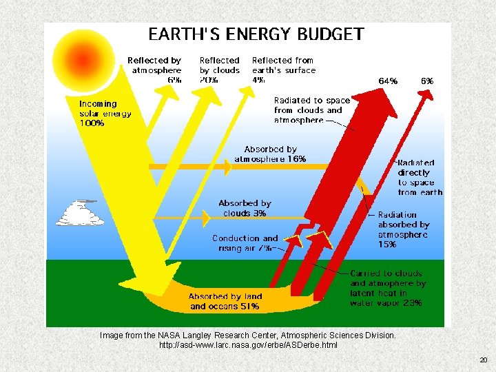
Image from the NASA Langley Research Center, Atmospheric Sciences Division. http: //asd-www. larc. nasa. gov/erbe/ASDerbe. html 20

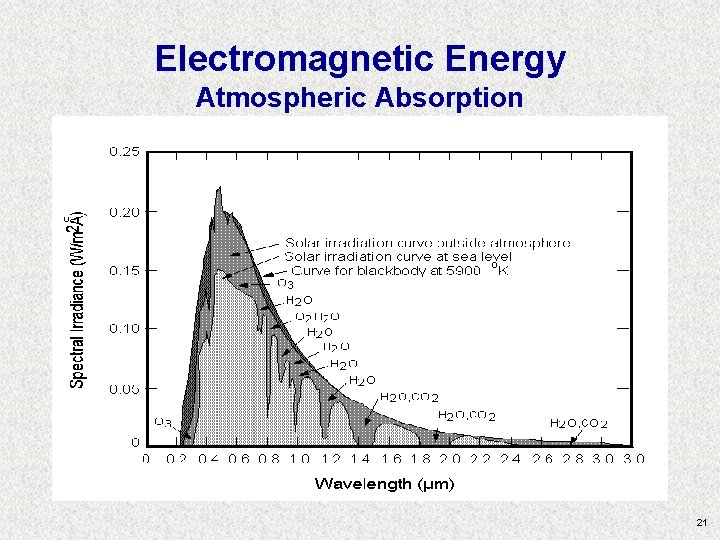
Electromagnetic Energy Atmospheric Absorption 21

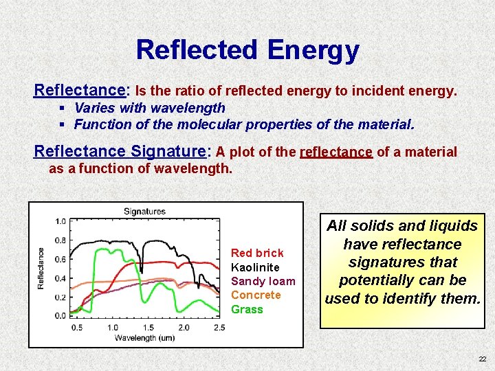
Reflected Energy Reflectance: Is the ratio of reflected energy to incident energy. § Varies with wavelength § Function of the molecular properties of the material. Reflectance Signature: A plot of the reflectance of a material as a function of wavelength. Red brick Kaolinite Sandy loam Concrete Grass All solids and liquids have reflectance signatures that potentially can be used to identify them. 22

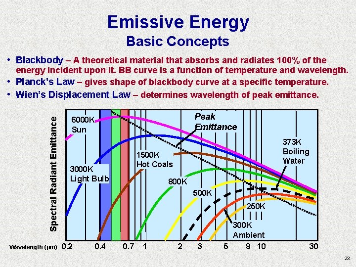
Emissive Energy Basic Concepts • Blackbody – A theoretical material that absorbs and radiates 100% of the Spectral Radiant Emittance • • energy incident upon it. BB curve is a function of temperature and wavelength. Planck’s Law – gives shape of blackbody curve at a specific temperature. Wien’s Displacement Law – determines wavelength of peak emittance. Wavelength (µm) Peak Emittance 6000 K Sun 373 K Boiling Water 1500 K Hot Coals 3000 K Light Bulb 800 K 500 K 250 K 0. 2 0. 4 0. 7 1 2 3 300 K Ambient 5 8 10 30 23

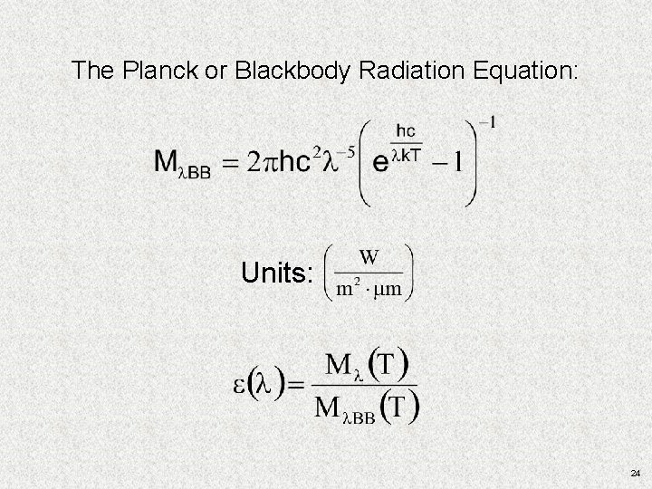
The Planck or Blackbody Radiation Equation: Units: 24

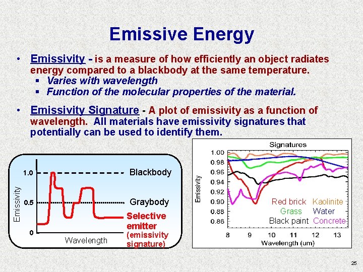
Emissive Energy • Emissivity - is a measure of how efficiently an object radiates energy compared to a blackbody at the same temperature. § Varies with wavelength § Function of the molecular properties of the material. • Emissivity Signature - A plot of emissivity as a function of Emissivity wavelength. All materials have emissivity signatures that potentially can be used to identify them. 1. 0 Blackbody 0. 5 Graybody 0 Selective emitter Wavelength Red brick Kaolinite Grass Water Black paint Concrete (emissivity signature) 25

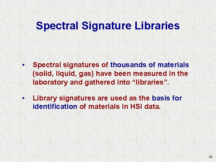
Spectral Signature Libraries • Spectral signatures of thousands of materials (solid, liquid, gas) have been measured in the laboratory and gathered into “libraries”. • Library signatures are used as the basis for identification of materials in HSI data. 26

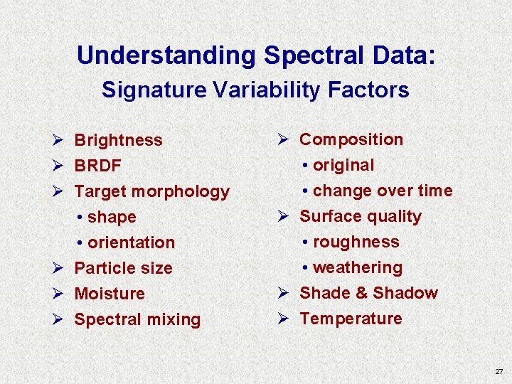
Understanding Spectral Data: Signature Variability Factors Ø Brightness Ø BRDF Ø Target morphology • shape • orientation Ø Particle size Ø Moisture Ø Spectral mixing Ø Composition • original • change over time Ø Surface quality • roughness • weathering Ø Shade & Shadow Ø Temperature 27

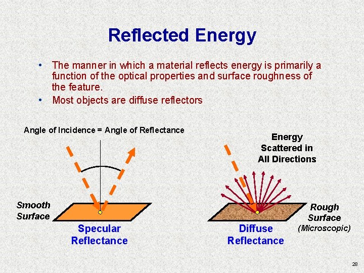
Reflected Energy • The manner in which a material reflects energy is primarily a function of the optical properties and surface roughness of the feature. • Most objects are diffuse reflectors Angle of Incidence = Angle of Reflectance Energy Scattered in All Directions Smooth Surface Specular Reflectance Diffuse Reflectance Rough Surface (Microscopic) 28

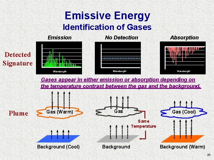
Emissive Energy Identification of Gases Emission No Detection Absorption Detected Signature Wavelength Gases appear in either emission or absorption depending on the temperature contrast between the gas and the background. Plume Gas (Warm) Gas (Cool) Same Temperature Background (Cool) Background (Warm) 29

Resolutions • Spatial Resolution • Radiometric Resolution • Temporal Resolution 30

HSI Fundamentals Summary • Hyperspectral remote sensing involves measuring energy in the Visible – LWIR portions of the electromagnetic spectrum. • Some of the measured energy is reflected from objects while some energy is emitted from objects. • Every material has a unique spectral signature. • Spectral image data are collected such that signatures can be extracted for material detection, classification, identification, characterization, and quantification. • Spectral, spatial, radiometric, and temporal resolution determine the capabilities of the remote sensing sensor/system. 31

Properties of the Data Cube • # of samples, lines, bands • Headers, preline, postline, footers, etc. • Data type • Interleaving (BIP, BIL, BSQ) • Byte order • Wavelengths, FWHM • Bad bands list • Band names (very optional) • The logical and physical data cube • The ENVI “. hdr” file • History file (it doesn’t exist) – keep notes! 32

An AVIRIS (NASA) HSI Image Cube 33

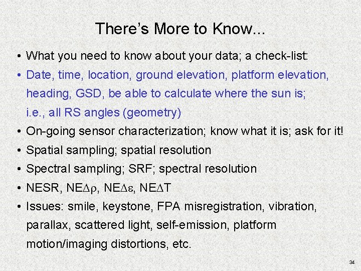
There’s More to Know. . . • What you need to know about your data; a check-list: • Date, time, location, ground elevation, platform elevation, heading, GSD, be able to calculate where the sun is; i. e. , all RS angles (geometry) • On-going sensor characterization; know what it is; ask for it! • Spatial sampling; spatial resolution • Spectral sampling; SRF; spectral resolution • NESR, NEDr, NEDe, NEDT • Issues: smile, keystone, FPA misregistration, vibration, parallax, scattered light, self-emission, platform motion/imaging distortions, etc. 34

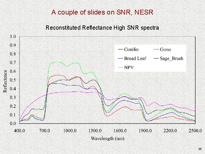
A couple of slides on SNR, NESR Reconstituted Reflectance High SNR spectra 35

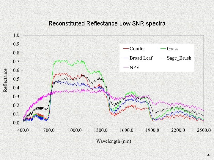
Reconstituted Reflectance Low SNR spectra 36

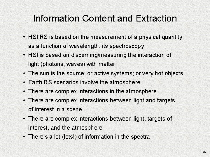
Information Content and Extraction • HSI RS is based on the measurement of a physical quantity as a function of wavelength: its spectroscopy • HSI is based on discerning/measuring the interaction of light (photons, waves) with matter • The sun is the source; or active systems; or very hot objects • Earth RS scenarios involve the atmosphere • There are complex interactions in the atmosphere • There are complex interactions between light and targets of interest in a scene • There are complex interactions between light, targets of interest, and the atmosphere • There’s a lot (lots!) of information in the spectra 37

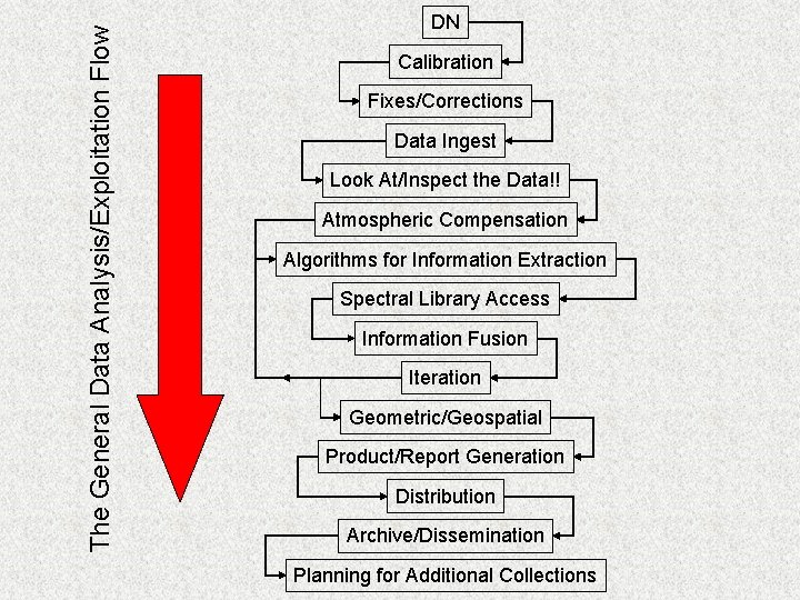
The General Data Analysis/Exploitation Flow DN Calibration Fixes/Corrections Data Ingest Look At/Inspect the Data!! Atmospheric Compensation Algorithms for Information Extraction Spectral Library Access Information Fusion Iteration Geometric/Geospatial Product/Report Generation Distribution Archive/Dissemination Planning for Additional Collections

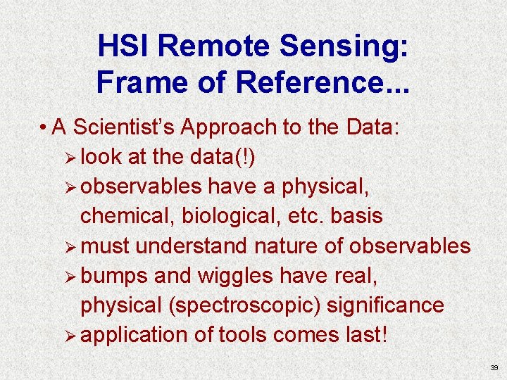
HSI Remote Sensing: Frame of Reference. . . • A Scientist’s Approach to the Data: Ø look at the data(!) Ø observables have a physical, chemical, biological, etc. basis Ø must understand nature of observables Ø bumps and wiggles have real, physical (spectroscopic) significance Ø application of tools comes last! 39

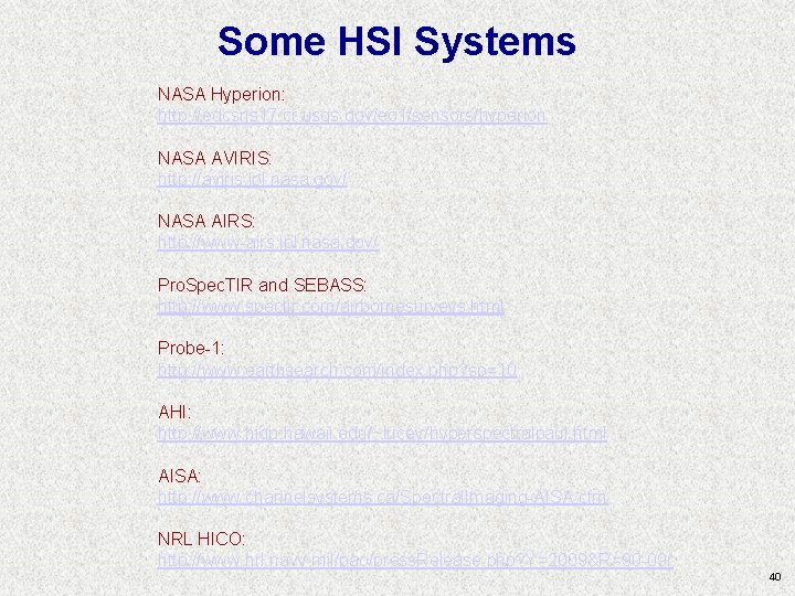
Some HSI Systems NASA Hyperion: http: //edcsns 17. cr. usgs. gov/eo 1/sensors/hyperion NASA AVIRIS: http: //aviris. jpl. nasa. gov/ NASA AIRS: http: //www-airs. jpl. nasa. gov/ Pro. Spec. TIR and SEBASS: http: //www. spectir. com/airbornesurveys. html Probe-1: http: //www. earthsearch. com/index. php? sp=10 AHI: http: //www. higp. hawaii. edu/~lucey/hyperspectralpaul. html AISA: http: //www. channelsystems. ca/Spectral. Imaging-AISA. cfm NRL HICO: http: //www. nrl. navy. mil/pao/press. Release. php? Y=2009&R=90 -09 r 40

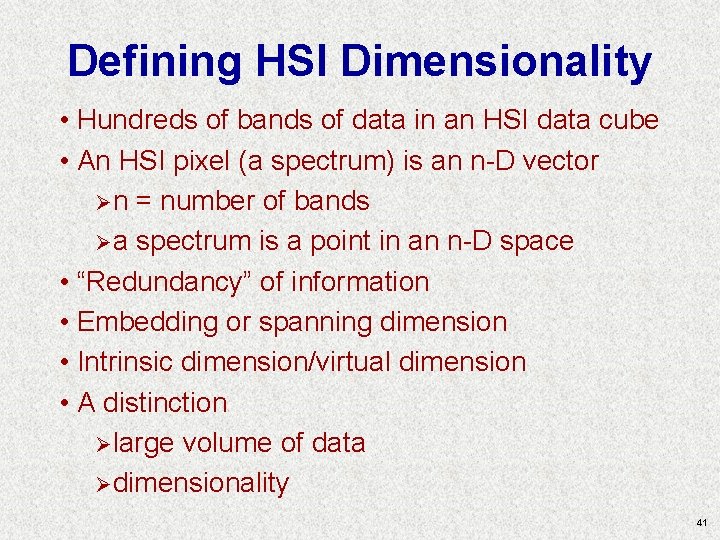
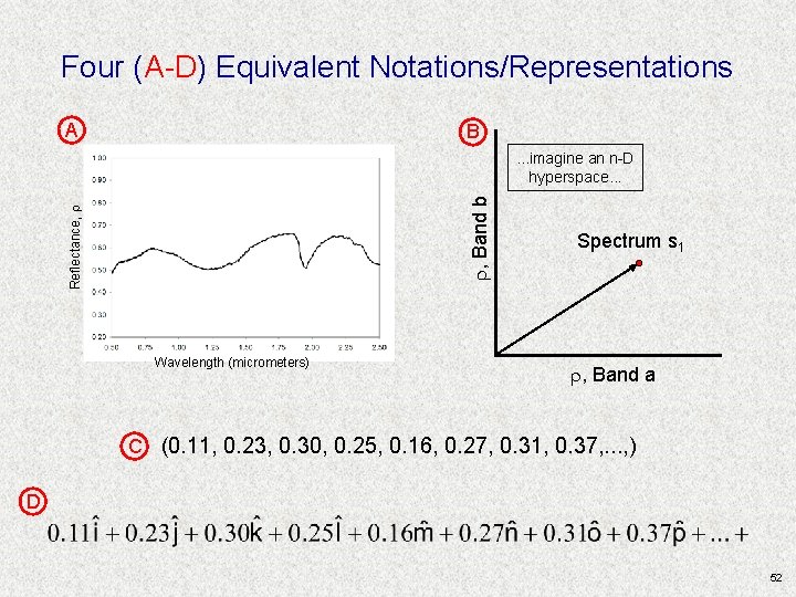
Defining HSI Dimensionality • Hundreds of bands of data in an HSI data cube • An HSI pixel (a spectrum) is an n-D vector Ø n = number of bands Ø a spectrum is a point in an n-D space • “Redundancy” of information • Embedding or spanning dimension • Intrinsic dimension/virtual dimension • A distinction Ø large volume of data Ø dimensionality 41

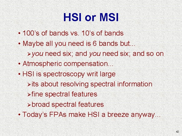
HSI or MSI • 100’s of bands vs. 10’s of bands • Maybe all you need is 6 bands but. . . Ø you need six; and so on • Atmospheric compensation. . . • HSI is spectroscopy writ large Ø its about resolving spectral information Ø fine spectral features Ø broad spectral features • Today’s FPAs make HSI a breeze anyway. . . 42

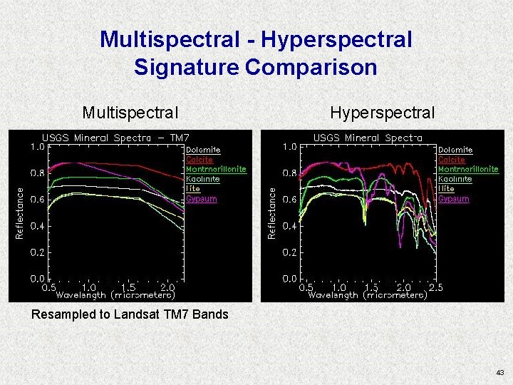
Multispectral - Hyperspectral Signature Comparison Multispectral Hyperspectral Resampled to Landsat TM 7 Bands 43

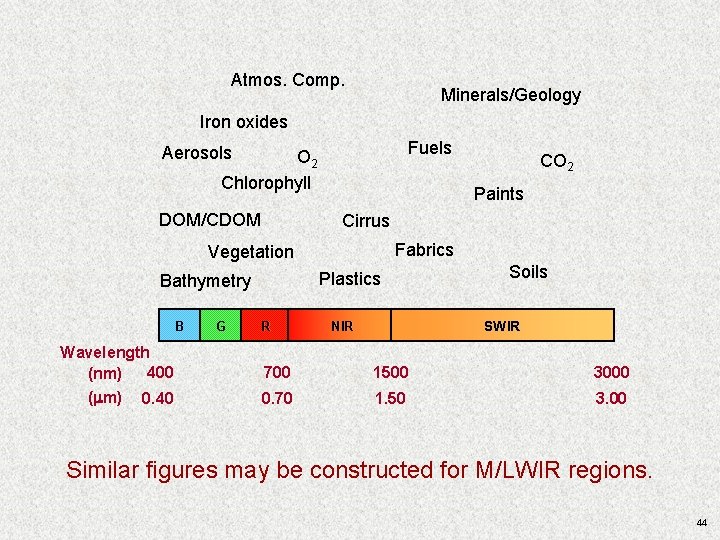
Atmos. Comp. Minerals/Geology Iron oxides Fuels Aerosols O 2 Chlorophyll DOM/CDOM Paints Cirrus Fabrics Vegetation Plastics Bathymetry B Wavelength 400 (nm) ( m) 0. 40 G CO 2 R Soils SWIR NIR 700 1500 3000 0. 70 1. 50 3. 00 Similar figures may be constructed for M/LWIR regions. 44

Thinking About Spectra; Thinking about HSI 45

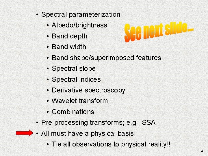
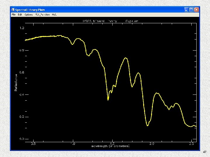
• Spectral parameterization • Albedo/brightness • Band depth • Band width • Band shape/superimposed features • Spectral slope • Spectral indices • Derivative spectroscopy • Wavelet transform • Combinations • Pre-processing transforms; e. g. , SSA • All must have a physical basis! • Tie all observations to physical reality!! 46

47

HSI Algorithms: An Introduction (Don’t Panic!!) 48

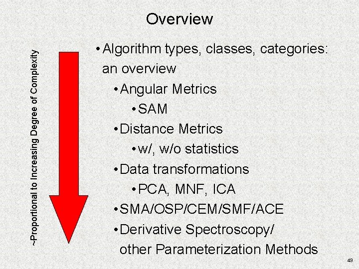
~Proportional to Increasing Degree of Complexity Overview • Algorithm types, classes, categories: an overview • Angular Metrics • SAM • Distance Metrics • w/, w/o statistics • Data transformations • PCA, MNF, ICA • SMA/OSP/CEM/SMF/ACE • Derivative Spectroscopy/ other Parameterization Methods 49

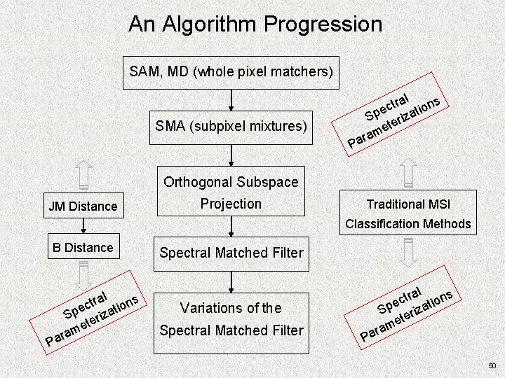
An Algorithm Progression SAM, MD (whole pixel matchers) ral ons t c i e Sp erizat et m ara SMA (subpixel mixtures) P Orthogonal Subspace JM Distance Projection Traditional MSI Classification Methods B Distance P ral ons t c i e Sp erizat et m ara Spectral Matched Filter Variations of the ral ons t c i e Sp erizat et m ara Spectral Matched Filter P 50

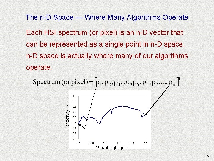
The n-D Space — Where Many Algorithms Operate Each HSI spectrum (or pixel) is an n-D vector that can be represented as a single point in n-D space is actually where many of our algorithms Reflectivity, r operate. Wavelength (mm) 51

Four (A-D) Equivalent Notations/Representations A B Reflectance, r r, Band b . . . imagine an n-D hyperspace. . . Wavelength (micrometers) Spectrum s 1 r, Band a C (0. 11, 0. 23, 0. 30, 0. 25, 0. 16, 0. 27, 0. 31, 0. 37, . . . , ) D 52

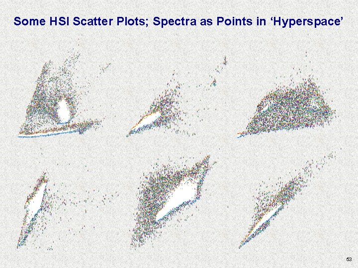
Some HSI Scatter Plots; Spectra as Points in ‘Hyperspace’ 53

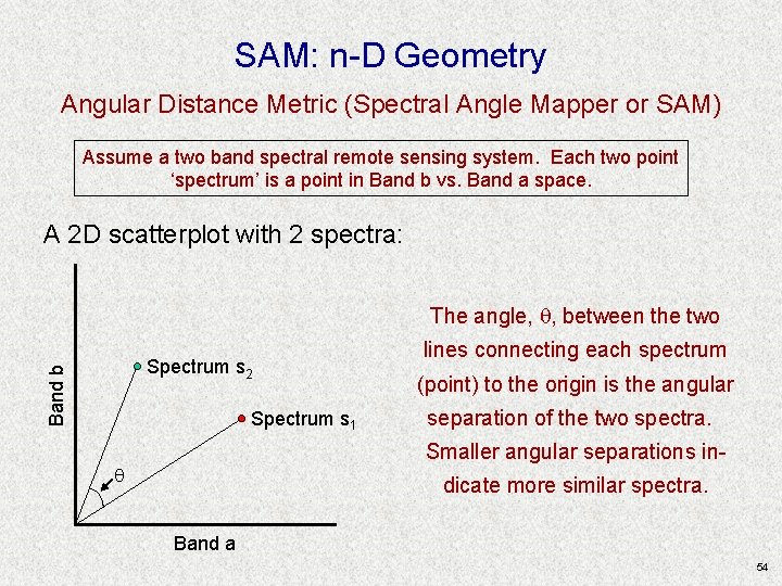
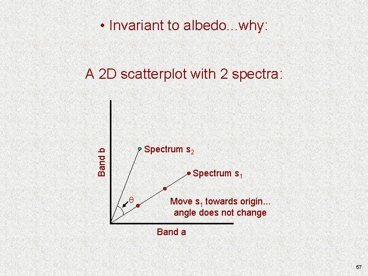
SAM: n-D Geometry Angular Distance Metric (Spectral Angle Mapper or SAM) Assume a two band spectral remote sensing system. Each two point ‘spectrum’ is a point in Band b vs. Band a space. A 2 D scatterplot with 2 spectra: The angle, , between the two Band b Spectrum s 2 Spectrum s 1 lines connecting each spectrum (point) to the origin is the angular separation of the two spectra. Smaller angular separations in- dicate more similar spectra. Band a 54

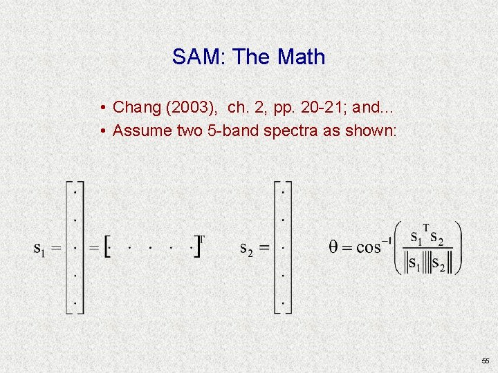
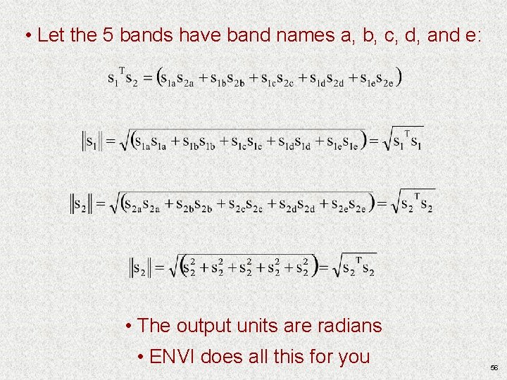
SAM: The Math • Chang (2003), ch. 2, pp. 20 -21; and. . . • Assume two 5 -band spectra as shown: 55

• Let the 5 bands have band names a, b, c, d, and e: • The output units are radians • ENVI does all this for you 56

• Invariant to albedo. . . why: A 2 D scatterplot with 2 spectra: Band b Spectrum s 2 Spectrum s 1 Move s 1 towards origin. . . angle does not change Band a 57

• Application strategies Ø Radiance, reflectance Ø Scaled values • A few comments on SAM and mixed pixels 58

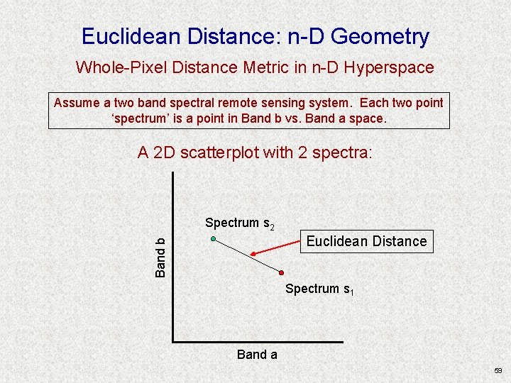
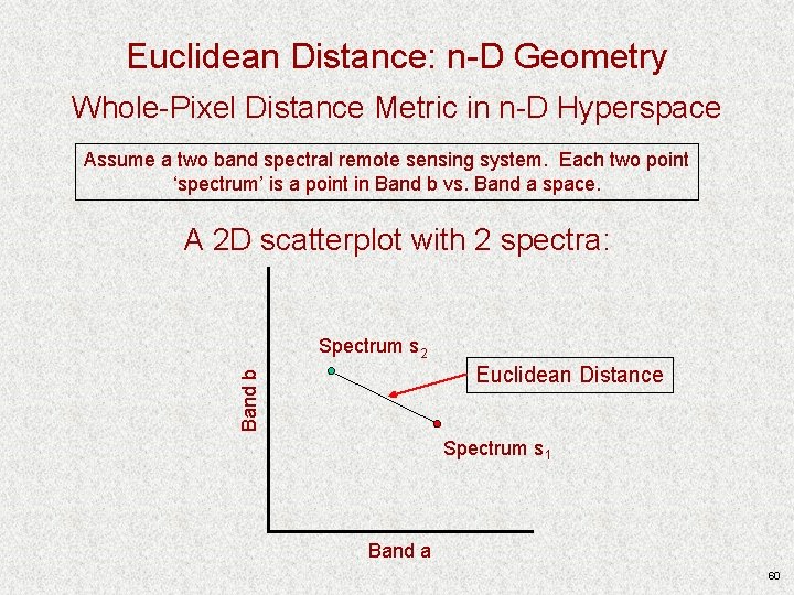
Euclidean Distance: n-D Geometry Whole-Pixel Distance Metric in n-D Hyperspace Assume a two band spectral remote sensing system. Each two point ‘spectrum’ is a point in Band b vs. Band a space. A 2 D scatterplot with 2 spectra: Spectrum s 2 Band b Euclidean Distance Spectrum s 1 Band a 59

Euclidean Distance: n-D Geometry Whole-Pixel Distance Metric in n-D Hyperspace Assume a two band spectral remote sensing system. Each two point ‘spectrum’ is a point in Band b vs. Band a space. A 2 D scatterplot with 2 spectra: Spectrum s 2 Band b Euclidean Distance Spectrum s 1 Band a 60

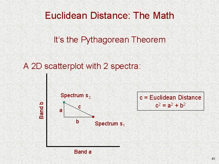
Euclidean Distance: The Math It’s the Pythagorean Theorem A 2 D scatterplot with 2 spectra: Band b Spectrum s 2 a c = Euclidean Distance c 2 = a 2 + b 2 c b Spectrum s 1 Band a 61

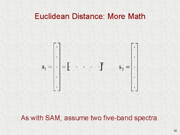
Euclidean Distance: More Math As with SAM, assume two five-band spectra. 62

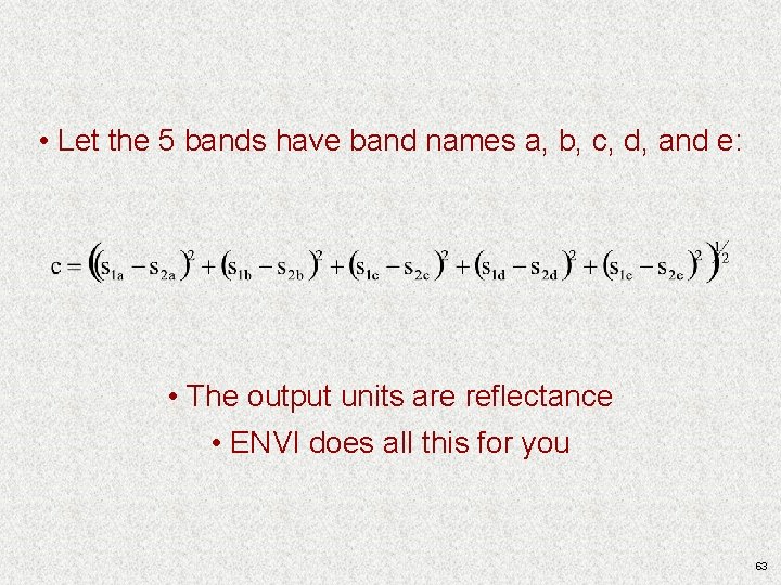
• Let the 5 bands have band names a, b, c, d, and e: • The output units are reflectance • ENVI does all this for you 63

• Application strategies Ø Radiance, reflectance Ø Scaled values • A few comments on Euclidean distance and mixed pixels 64

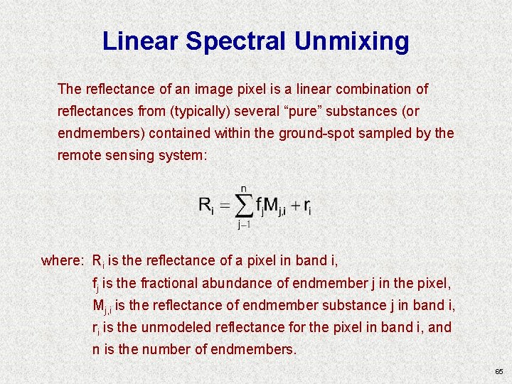
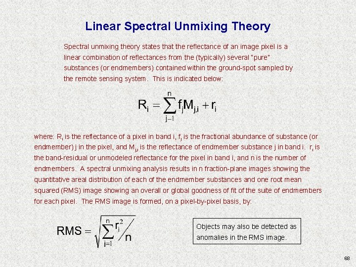
Linear Spectral Unmixing The reflectance of an image pixel is a linear combination of reflectances from (typically) several “pure” substances (or endmembers) contained within the ground-spot sampled by the remote sensing system: where: Ri is the reflectance of a pixel in band i, fj is the fractional abundance of endmember j in the pixel, Mj, i is the reflectance of endmember substance j in band i, ri is the unmodeled reflectance for the pixel in band i, and n is the number of endmembers. 65

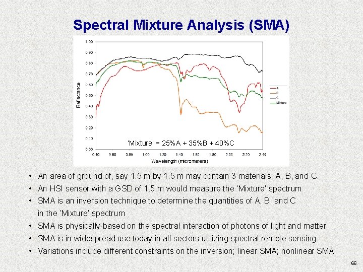
Spectral Mixture Analysis (SMA) ‘Mixture’ = 25%A + 35%B + 40%C • An area of ground of, say 1. 5 m by 1. 5 m may contain 3 materials: A, B, and C. • An HSI sensor with a GSD of 1. 5 m would measure the ‘Mixture’ spectrum • SMA is an inversion technique to determine the quantities of A, B, and C in the ‘Mixture’ spectrum • SMA is physically-based on the spectral interaction of photons of light and matter • SMA is in widespread use today in all sectors utilizing spectral remote sensing • Variations include different constraints on the inversion; linear SMA; nonlinear SMA 66

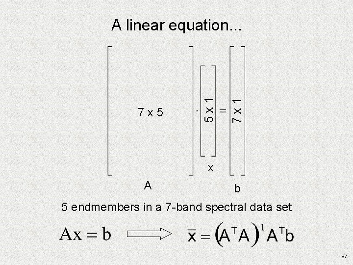
7 x 1 7 x 5 5 x 1 A linear equation. . . x A b 5 endmembers in a 7 -band spectral data set 67

Linear Spectral Unmixing Theory Spectral unmixing theory states that the reflectance of an image pixel is a linear combination of reflectances from the (typically) several “pure” substances (or endmembers) contained within the ground-spot sampled by the remote sensing system. This is indicated below: where: Ri is the reflectance of a pixel in band i, fj is the fractional abundance of substance (or endmember) j in the pixel, and Mj, i is the reflectance of endmember substance j in band i. ri is the band-residual or unmodeled reflectance for the pixel in band i, and n is the number of endmembers. A spectral unmixing analysis results in n fraction-plane images showing the quantitative areal distribution of each of the endmember substances and one root mean squared (RMS) image showing an overall or global goodness of fit of the suite of endmembers for each pixel. The RMS image is formed, on a pixel-by-pixel basis, by: Objects may also be detected as anomalies in the RMS image. 68

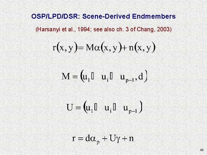
OSP/LPD/DSR: Scene-Derived Endmembers (Harsanyi et al. , 1994; see also ch. 3 of Chang, 2003) 69

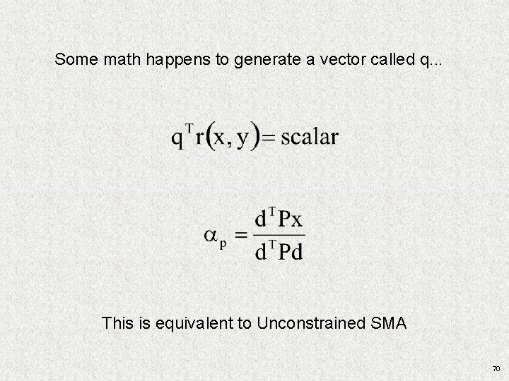
Some math happens to generate a vector called q. . . This is equivalent to Unconstrained SMA 70

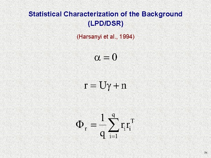
Statistical Characterization of the Background (LPD/DSR) (Harsanyi et al. , 1994) 71

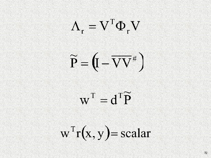
72

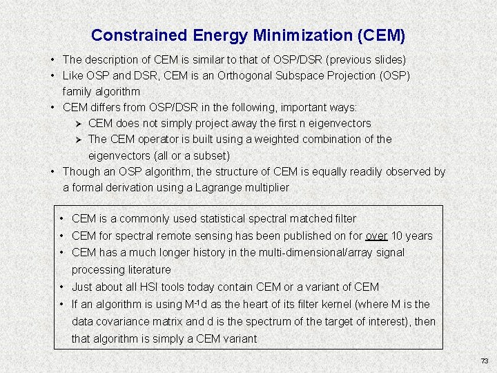
Constrained Energy Minimization (CEM) • The description of CEM is similar to that of OSP/DSR (previous slides) • Like OSP and DSR, CEM is an Orthogonal Subspace Projection (OSP) family algorithm • CEM differs from OSP/DSR in the following, important ways: Ø CEM does not simply project away the first n eigenvectors Ø The CEM operator is built using a weighted combination of the eigenvectors (all or a subset) • Though an OSP algorithm, the structure of CEM is equally readily observed by a formal derivation using a Lagrange multiplier • CEM is a commonly used statistical spectral matched filter • CEM for spectral remote sensing has been published on for over 10 years • CEM has a much longer history in the multi-dimensional/array signal processing literature • Just about all HSI tools today contain CEM or a variant of CEM • If an algorithm is using M-1 d as the heart of its filter kernel (where M is the data covariance matrix and d is the spectrum of the target of interest), then that algorithm is simply a CEM variant 73

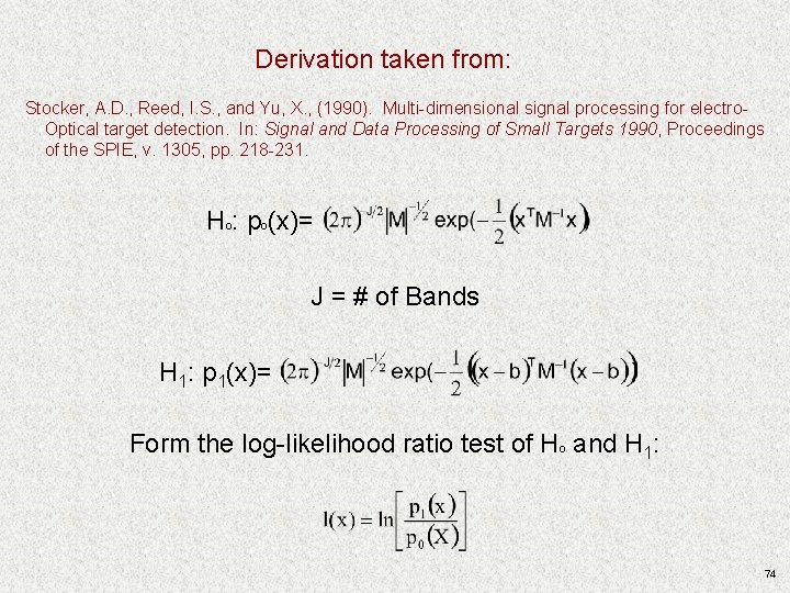
Derivation taken from: Stocker, A. D. , Reed, I. S. , and Yu, X. , (1990). Multi-dimensional signal processing for electro. Optical target detection. In: Signal and Data Processing of Small Targets 1990, Proceedings of the SPIE, v. 1305, pp. 218 -231. Hº: pº(x)= J = # of Bands H 1: p 1(x)= Form the log-likelihood ratio test of Hº and H 1: 74

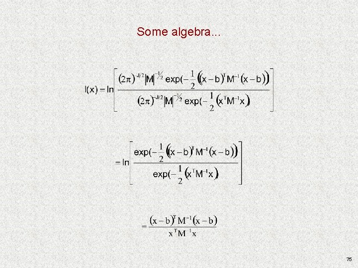
Some algebra. . . 75

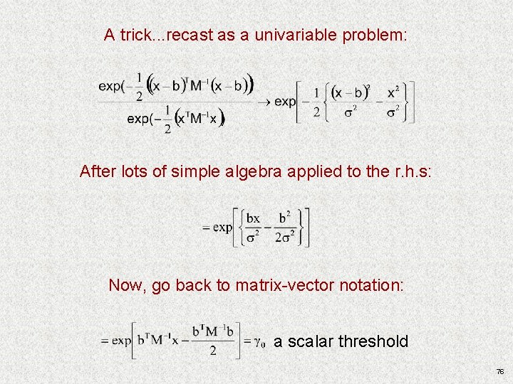
A trick. . . recast as a univariable problem: After lots of simple algebra applied to the r. h. s: Now, go back to matrix-vector notation: a scalar threshold 76

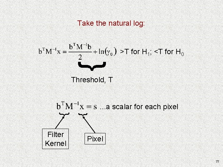
Take the natural log: { >T for H 1; <T for H 0 Threshold, T Filter Kernel { { . . . a scalar for each pixel Pixel 77

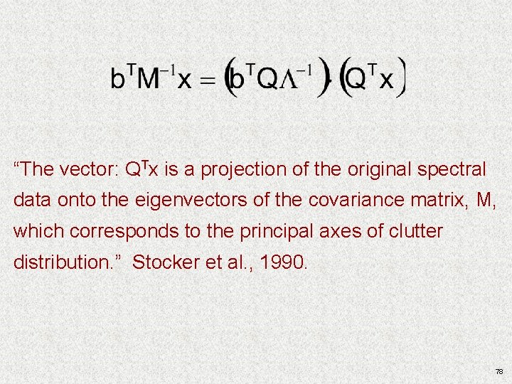
“The vector: QTx is a projection of the original spectral data onto the eigenvectors of the covariance matrix, M, which corresponds to the principal axes of clutter distribution. ” Stocker et al. , 1990. 78

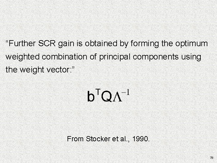
“Further SCR gain is obtained by forming the optimum weighted combination of principal components using the weight vector: ” From Stocker et al. , 1990. 79

Its Important to Note That. . . Today’s HSI algorithms can also benefit from 1) spatial and spectral subsetting; 2) hierarchical application of techniques; 3) other. . . 80

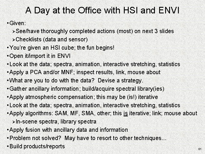
A Day at the Office with HSI and ENVI • Given: ØSee/have thoroughly completed actions (most) on next 3 slides ØChecklists (data and sensor) • You’re given an HSI cube; the fun begins! • Open it/import it in ENVI • Look at the data; spectra, animation, interactive stretching, statistics • Apply a PCA and/or MNF; inspect results, link, mouse about • What are you to do with the data? Devise a strategy. • Gather ancillary information; build/acquire spectral library(ies) • Apply atmospheric compensation; this may be (is!) iterative • Look at the data; spectra, animation, interactive stretching, statistics • Apply algorithms: SAM, MF, SMA, other; this is iterative; link; mouse about ØIn-scene spectra, library spectra • Apply fusion with ancillary data and information • Problem not solved? May have to resort to other techniques. . . • Build products/reports 81

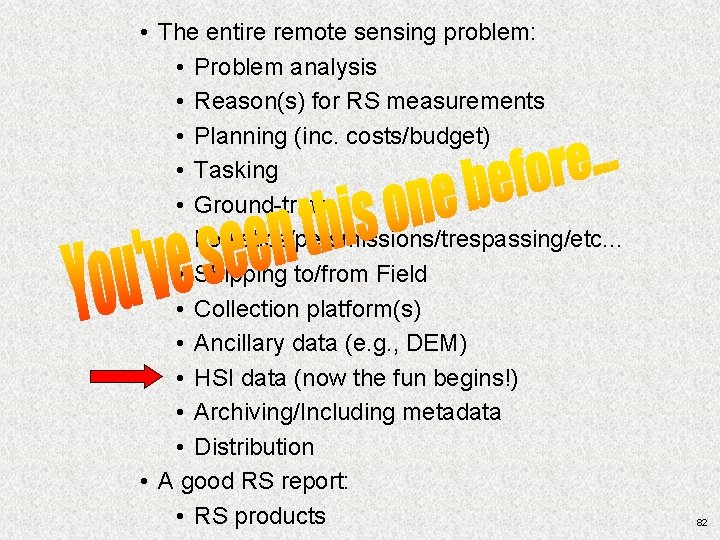
• The entire remote sensing problem: • Problem analysis • Reason(s) for RS measurements • Planning (inc. costs/budget) • Tasking • Ground-truth • Logistics/persmissions/trespassing/etc. . . • Shipping to/from Field • Collection platform(s) • Ancillary data (e. g. , DEM) • HSI data (now the fun begins!) • Archiving/Including metadata • Distribution • A good RS report: • RS products 82

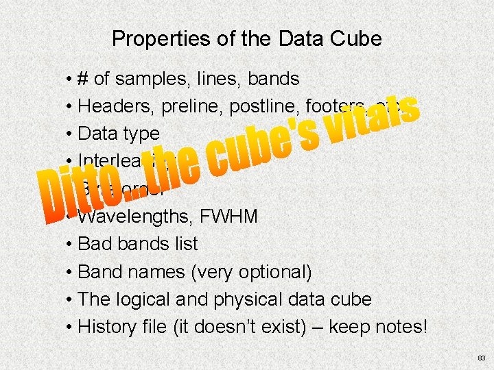
Properties of the Data Cube • # of samples, lines, bands • Headers, preline, postline, footers, etc. • Data type • Interleaving • Byte order • Wavelengths, FWHM • Bad bands list • Band names (very optional) • The logical and physical data cube • History file (it doesn’t exist) – keep notes! 83

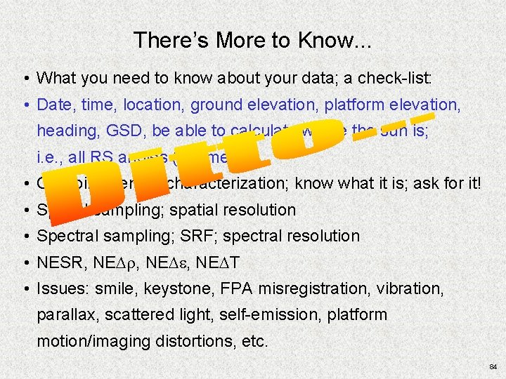
There’s More to Know. . . • What you need to know about your data; a check-list: • Date, time, location, ground elevation, platform elevation, heading, GSD, be able to calculate where the sun is; i. e. , all RS angles (geometry) • On-going sensor characterization; know what it is; ask for it! • Spatial sampling; spatial resolution • Spectral sampling; SRF; spectral resolution • NESR, NEDr, NEDe, NEDT • Issues: smile, keystone, FPA misregistration, vibration, parallax, scattered light, self-emission, platform motion/imaging distortions, etc. 84

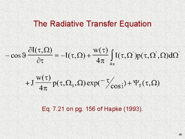
Introduction to Radiative Transfer Theory 85

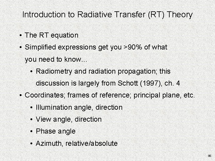
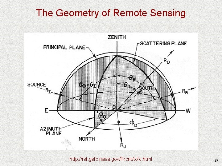
Introduction to Radiative Transfer (RT) Theory • The RT equation • Simplified expressions get you >90% of what you need to know… • Radiometry and radiation propagation; this discussion is largely from Schott (1997), ch. 4 • Coordinates; frames of reference; principal plane, etc. • Illumination angle, direction • View angle, direction • Phase angle • Azimuth, relative/absolute 86

The Geometry of Remote Sensing http: //rst. gsfc. nasa. gov/Front/tofc. html 87

The Radiative Transfer Equation Eq. 7. 21 on pg. 156 of Hapke (1993). 88

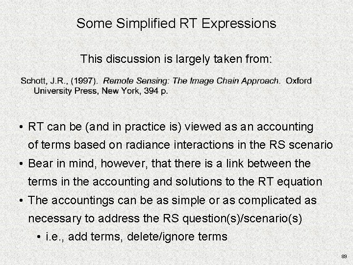
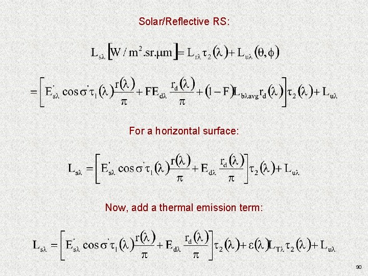
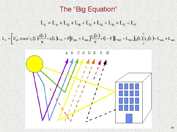
Some Simplified RT Expressions This discussion is largely taken from: • RT can be (and in practice is) viewed as an accounting of terms based on radiance interactions in the RS scenario • Bear in mind, however, that there is a link between the terms in the accounting and solutions to the RT equation • The accountings can be as simple or as complicated as necessary to address the RS question(s)/scenario(s) • i. e. , add terms, delete/ignore terms 89

Solar/Reflective RS: For a horizontal surface: Now, add a thermal emission term: 90

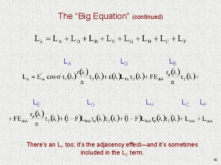
The “Big Equation” 91

The “Big Equation” (continued) LA LE LD LG LB LH LC LF There’s an LI, too; it’s the adjacency effect—and it’s sometimes included in the LC term. 92

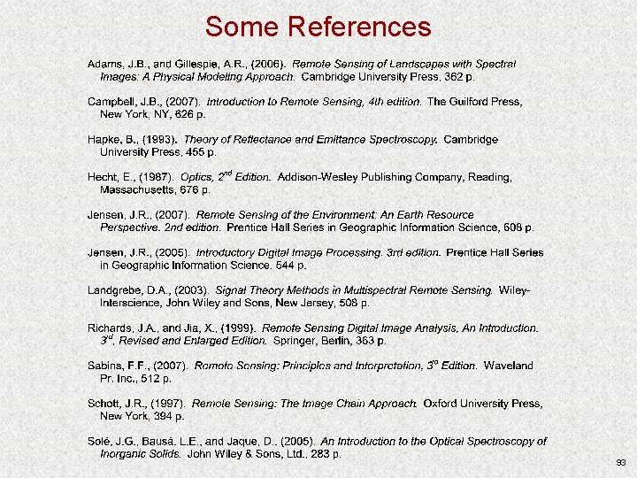
Some References 93