Einfhrung in Web und DataScience Prof Dr Ralf

Einführung in Web- und Data-Science Prof. Dr. Ralf Möller Universität zu Lübeck Institut für Informationssysteme
 –")
Repräsentation von Funktionen. . . • … durch Perzeptrons – Ein-Ebenen-Netzwerk (Linearer Klassifikator) – Mehrebenen-Netzwerke – Lernregel Fehlerrückführung (Backpropagation) Frank Rosenblatt, The Perceptron--a perceiving and recognizing automaton. Report 85 -460 -1, Cornell Aeronautical Laboratory, 1957
: sonst")
Perzeptron sonst Manchmal einfacher geschrieben als (Ann. : x 0 = 1): sonst

Entscheidungslinie eines Perzeptrons Repräsentiert lineare Funktion y = mx + b Was machen die Gewichte? Verallgemeinerung auf Entscheidungsebenen möglich Vgl. : Warren Mc. Culloch und William Pitts: A logical calculus of the ideas immanent in nervous activity. In: Bulletin of Mathematical Biophysics, Bd. 5, S. 115– 133, 1943

Trennlinien • Wenn w 2 x 2 + w 1 x 1 + w 0 > 0, dann wird für (x 1, x 2) ein (+) vergeben. • w 2 x 2 + w 1 x 1 + w 0 = 0 ist Trennlinie. Warum? • Es wird die Gerade x 2 = -w 1/w 2 x 1 - w 0/w 2 als Trennlinie verwendet. • Wir betrachten y = mx + b • Bedingung lautet: y – mx - b > 0 • Wähle m=1 und b positiv. Dann betrachte (x, y) = (0, 2 b). Das liegt über der Geraden. • 2 b – 0 – b > 0 • Also wird (0, 2 b) mit 1 bewertet (+) 5

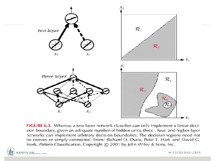
Lassen sich alle Funktionen repräsentatieren? • Kann die Fehlerfunktion immer sinnvoll minimiert werden? • XOR-Problem – Einführung weiterer Dimensionen • Erweiterung der Daten? – Besser: Einführung weiterer Ebenen im Netz Marvin Minsky and Seymour Papert (2 nd edition with corrections, first edition 1969) Perceptrons: An Introduction to Computational Geometry, The MIT Press, Cambridge MA, 1972

Ein Anwendungsbeispiel Das folgende Netz soll Ziffern von 0 bis 9 erkennen. Dafür wird zunächst das Eingabefeld in 8 x 15 Elemente aufgeteilt: Wie können wir die Parameter automatisch so bestimmen, dass geschriebene Ziffern erkannt und als Ausgabe y ausgegeben werden? Die geschriebene Ziffer wird in eine Folge von Nullen und Einsen umgewandelt, wobei 0 für leere und 1 für übermalte Rasterpunkte steht:

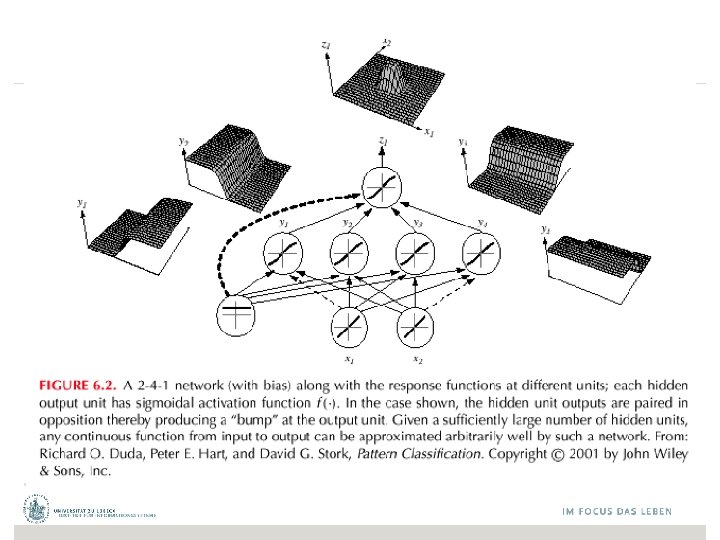
Verwendung kontinuierlicher Funktionen ist die Sigmoid-Funktion
 W 3 1. 4 David")
-0. 06 W 1 -2. 5 W 2 f(x) W 3 1. 4 David Corne: Open Courseware
 0. 002 x = -0.")
-0. 06 2. 7 -2. 5 -8. 6 f(x) 0. 002 x = -0. 06× 2. 7 + 2. 5× 8. 6 + 1. 4× 0. 002 = 21. 34 1. 4 David Corne: Open Courseware
 Eigenschaft: (Gradient) • Wir können den Gradienten")
Sigmoid-Einheit ist die Sigmoid-Funktion (auch: logistische Funktion) Eigenschaft: (Gradient) • Wir können den Gradienten verwenden, um die Einheit anzupassen • Wir kommen gleich darauf zurück

Mehr-Ebenen Netze von Sigmoid-Einheiten
 AND")
Z = x 1 XOR x 2 = (x 1 OR x 2) AND NOT(x 1 AND x 2)

Netztopologien Feed. Forward-Netze: Gerichtete Verbindungen nur von niedrigen zu höheren Schichten Feed. Back-Netze (rekurrente Netze): Verbindungen zwischen allen Schichten möglich (Abrollen) FB-Netz mit Lateralverbindungen FF-Netz erster Ordnung FF-Netz zweiter Ordnung FB-Netz mit direkter Rückkopplung © Stefan Hartmann

Netzwerk von Perzeptrons • Perzeptron: Eingabefunktio n Aktivierungsfunktion Ausgabefunktion • Was muss ich vor dem Lernen/Trainieren bestimmen? – Netzwerk-Topologie? – Perzeptron bezogen? 17

Die Eingabefunktion • © Stefan Hartmann

Die Aktivierungsfunktion • Schwellenwert, häufig 0 Spezialfall: Sigmoid: T=1 © Stefan Hartmann

Die Ausgabefunktion • © Stefan Hartmann

Einstellen der Gewichte mit Trainingsdaten… Fields 1. 4 2. 7 3. 8 3. 4 6. 4 2. 8 4. 1 0. 1 etc … 1. 9 3. 2 1. 7 0. 2 class 0 0 1 0 David Corne: Open Courseware

Anlernen des Netzwerks Fields 1. 4 2. 7 3. 8 3. 4 6. 4 2. 8 4. 1 0. 1 etc … 1. 9 3. 2 1. 7 0. 2 class 0 0 1 0 Eingabe David Corne: Open Courseware Perzeptrons Ausgabe

Trainingsdaten Fields 1. 4 2. 7 3. 8 3. 4 6. 4 2. 8 4. 1 0. 1 etc … 1. 9 3. 2 1. 7 0. 2 class 0 0 1 0 Initialisierung mit zufälligen Gewichten David Corne: Open Courseware

Trainingsdaten Fields 1. 4 2. 7 3. 8 3. 4 6. 4 2. 8 4. 1 0. 1 etc … 1. 9 3. 2 1. 7 0. 2 class 0 0 1 0 Präsentierung eines Trainingsdatensatzes 1. 4 2. 7 1. 9 David Corne: Open Courseware

Trainingsdaten Fields 1. 4 2. 7 3. 8 3. 4 6. 4 2. 8 4. 1 0. 1 etc … 1. 9 3. 2 1. 7 0. 2 class 0 0 1 0 Durchpropagierung zur Ausgabe 1. 4 2. 7 1. 9 David Corne: Open Courseware 0. 8

Trainingsdaten Fields 1. 4 2. 7 3. 8 3. 4 6. 4 2. 8 4. 1 0. 1 etc … 1. 9 3. 2 1. 7 0. 2 class 0 0 1 0 Vergleich mit der Zielausgabe 1. 4 2. 7 0. 8 0 1. 9 David Corne: Open Courseware Fehler 0. 8

Trainingsdaten Fields 1. 4 2. 7 3. 8 3. 4 6. 4 2. 8 4. 1 0. 1 etc … 1. 9 3. 2 1. 7 0. 2 class 0 0 1 0 Anpassen der Gewichte gemäß Fehler 1. 4 2. 7 0. 8 0 1. 9 David Corne: Open Courseware Fehler 0. 8

Trainingsdaten Fields 1. 4 2. 7 3. 8 3. 4 6. 4 2. 8 4. 1 0. 1 etc … 1. 9 3. 2 1. 7 0. 2 class 0 0 1 0 Präsentierung eines Trainingsdatensatzes 6. 4 2. 8 1. 7 David Corne: Open Courseware

Trainingsdaten Fields 1. 4 2. 7 3. 8 3. 4 6. 4 2. 8 4. 1 0. 1 etc … 1. 9 3. 2 1. 7 0. 2 class 0 0 1 0 Durchpropagierung zur Ausgabe 6. 4 2. 8 1. 7 David Corne: Open Courseware 0. 9

Trainingsdaten Fields 1. 4 2. 7 3. 8 3. 4 6. 4 2. 8 4. 1 0. 1 etc … 1. 9 3. 2 1. 7 0. 2 class 0 0 1 0 Vergleich mit der Zielausgabe 6. 4 2. 8 0. 9 1 1. 7 David Corne: Open Courseware Fehler -0. 1

Trainingsdaten Fields 1. 4 2. 7 3. 8 3. 4 6. 4 2. 8 4. 1 0. 1 etc … 1. 9 3. 2 1. 7 0. 2 class 0 0 1 0 Anpassen der Gewichte gemäß Fehler 6. 4 2. 8 0. 9 1 1. 7 David Corne: Open Courseware Fehler -0. 1

Trainingsdaten Fields 1. 4 2. 7 3. 8 3. 4 6. 4 2. 8 4. 1 0. 1 etc … 1. 9 3. 2 1. 7 0. 2 class 0 0 1 0 Und so weiter …. 6. 4 2. 8 0. 9 1 1. 7 Fehler -0. 1 Wiederhole tausend-, vielleicht millionenmal – jedesmal mit einer zufälligen Trainingsinstanz und einer kleinen Anpassung der Gewichte Verfahren zur Gewichtsanpassung müssen Fehler minimieren David Corne: Open Courseware
 • Frank Rosenblatt, The Perceptron--a perceiving and recognizing automaton.")
Eine Ebene: Perzeptron-Lernregel (Delta. Lernregel) • Frank Rosenblatt, The Perceptron--a perceiving and recognizing automaton. Report 85 -460 -1, Cornell Aeronautical Laboratory, 1957 33

Begründung für die Delta-Regel •

Absteigender Gradient • 35

Gradient • 36
 • 37")
Absteigender Gradient (Forts. ) • 37

Algorithmus für eine Gewichtsanpassung • 38

Perzeptron-Lernregel Man kann zeigen, dass der Vorgang konvergiert, … • . . . wenn die Daten linear separierbar sind • . . . und �� genügend klein gewählt wird Schon früher untersucht: D. Hebb: The organization of behavior. A neuropsychological theory. Erlbaum Books, Mahwah, N. J. , 1949 Netzwerke daher von manchen als künstliche neuronale Netze bezeichnet Später für mehrschichtige Netze erweitert (Deep Learning): Fehlerrückführung durch mehrere Ebenen (Backpropagation)

Aktivierung: Re. LU Takes a real-valued number and thresholds it at zero http: //adilmoujahid. com/images/activation. png Most Deep Networks use Re. LU nowadays � Trains much faster • accelerates the convergence of SGD • due to linear, non-saturating form � Less expensive operations • compared to sigmoid/tanh (exponentials etc. ) • implemented by simply thresholding a matrix at zero � More expressive � Prevents the gradient vanishing problem
 during training • Each")
Regularization Dropout • Randomly drop units (along with their connections) during training • Each unit retained with fixed probability p, independent of other units • Hyper-parameter p to be chosen (tuned) Srivastava, Nitish, et al. "Dropout: a simple way to prevent neural networks from overfitting. " Journal of machine learning research (2014) L 2 = weight decay • Regularization term that penalizes big weights, added to the objective • Weight decay value determines how dominant regularization is during gradient computation • Big weight decay coefficient big penalty for big weights Early-stopping • Use validation error to decide when to stop training • Stop when monitored quantity has not improved after n subsequent epochs • n is called patience
y j Cross-entropy")
Softmax output layer Softmax Network outputs a probability distribution! Δwij = (yi-zi)y j Cross-entropy loss after a softmax layer gives a very simple, numerically stable gradient 42

Perspektive der Entscheidungsgrenzenanpassung Zufällige Initialgewichte David Corne: Open Courseware

Perspektive der Entscheidungsgrenzenanpassung Verwenden einer Trainingsinstanz / Anpassung der Gewicht David Corne: Open Courseware

Perspektive der Entscheidungsgrenzenanpassung Verwenden einer Trainingsinstanz / Anpassung der Gewicht David Corne: Open Courseware

Perspektive der Entscheidungsgrenzenanpassung Verwenden einer Trainingsinstanz / Anpassung der Gewicht David Corne: Open Courseware

Perspektive der Entscheidungsgrenzenanpassung Verwenden einer Trainingsinstanz / Anpassung der Gewicht David Corne: Open Courseware

Perspektive der Entscheidungsgrenzenanpassung Und schließlich…. David Corne: Open Courseware

Fehler bei einer ungeeigneten Trainingsmenge Zu viele Trainingsbeispiele: Zu wenig Trainingsbeispiele: das Netz hat „auswendig gelernt“ keine richtige Klassifikation © Stefan Hartmann

Lernverfahren: Resümee • Epoche: einmalige Verwendung des gesamten Datensatzes – Manchmal zu groß • Batch: Zerlegung eines Datensatzes in Teilmengen – Für jede Teilmenge: Passe Gewichte an – Anzahl der Teilmengen: #Iterationen • Tausende von kleinen Anpassungen, jede macht das Netz besser für die letzte Eingabe (aber vielleicht schlechter für frühere Eingaben) • Verwende mehrere Epochen • Wieviele Epochen? Batches? – Ausprobieren • Durch verdammtes Glück kommt oft eine Funktion heraus, die gut genug in Anwendungen funktioniert

Word-Word Associations in Document Retrieval Recap bag-of-words approaches • Client profiles, TF-IDF Words are not independent of each other Need to represent some aspects of word semantics Church, K. W. , Hanks, P. : Word association norms mutual information, and lexicography. Comput. Linguist. 1(1), 22– 29, 1990 51
 Mutual Information: PMI • Measure of association used in information theory and statistics")
Point(wise) Mutual Information: PMI • Measure of association used in information theory and statistics • Positive PMI: PPMI(x, y) = max( pmi(x, y), 0 ) • Quantifies the discrepancy between the probability of their coincidence given their joint distribution and their individual distributions, assuming independence • Finding collocations and associations between words • Countings of occurrences and co-occurrences of words in a text corpus can be used to approximate the probabilities p(x) or p(y) and p(x, y) respectively [Wikipedia] 52

PMI – Example • Counts of pairs of words getting the most and the least PMI scores in the first 50 millions of words in Wikipedia (dump of October 2015) • Filtering by 1, 000 or more co-occurrences. • The frequency of each count can be obtained by dividing its value by 50, 000, 952. (Note: natural log is used to calculate the PMI values in this example, instead of log base 2) [Wikipedia] 53
 54")
PMI – Co-occurrence Matrix Count(w, context) 54

Embedding Approaches to Word Semantics • Represent each word with a low-dimensional vector • Word similarity = vector similarity • Key idea: Predict surrounding words of every word 55

Represent the meaning of words – word 2 vec • 2 basic structural models: – Continuous Bag of Words (CBOW): use a window of words to predict the middle word – Skip-gram (SG): use a word to predict the surrounding ones in window. 56

Word 2 vec – Continuous Bag of Word • E. g. “The cat <sat> on floor” – Window size = 2 the cat sat on floor 57

Input layer 0 Index of cat in vocabulary 1 0 0 cat 0 Hidden layer Output layer 0 one-hot vector 0 0 … 0 0 0 on 0 0 1 0 … 1 0 sat one-hot vector 0 0 … 0 58

We must learn W and W’ Input layer 0 1 0 0 cat 0 Hidden layer Output layer 0 V-dim 0 0 … 0 0 0 0 1 0 … 1 on sat N-dim 0 V-dim 0 0 V-dim … 0 N will be the size of word vector 59

Deep Learning • Hidden layer represents feature space – Making explicit features in the data… – … that are relevant for a certain task • Determine features automatically – Learning suitable mappings into feature space • Deep learning also known as representation learning 60

0. 1 2. 4 1. 6 1. 8 0. 5 0. 9 … Input layer 0 1 0 0 xcat V-dim … … 3. 2 0. 5 2. 6 1. 4 2. 9 1. 5 3. 6 … … … 6. 1 … … … … … 0. 6 1. 8 2. 7 1. 9 2. 4 2. 0 … … … 1. 2 1 0 0 0 0 … 0 0 2. 4 2. 6 … … 1. 8 Output layer 0 0 0 … 0 0 + 0 0 1 0 … 1 0 0 sat 0 0 xon 0 Hidden layer V-dim N-dim 0 V-dim … 0 61

0. 1 2. 4 1. 6 1. 8 0. 5 0. 9 … Input layer 0 1 0 0 xcat V-dim … … 3. 2 0. 5 2. 6 1. 4 2. 9 1. 5 3. 6 … … … 6. 1 … … … … … 0. 6 1. 8 2. 7 1. 9 2. 4 2. 0 … … … 1. 2 0 0 1 0 0 0 … 0 0 1. 8 2. 9 … … 1. 9 Output layer 0 0 0 … 0 0 + 0 0 1 0 … 1 0 0 sat 0 0 xon 0 Hidden layer V-dim N-dim 0 V-dim … 0 62

Input layer 0 1 0 0 cat 0 Hidden layer Output layer 0 V-dim 0 0 … 0 0 0 0 on 0 1 0 … 1 0 0 N-dim 0 0 V-dim … 0 N will be the size of word vector 63
![Logistic function [Wikipedia] 64](http://slidetodoc.com/presentation_image_h2/a394ad0525747c586803efb550f77fd3/image-64.jpg "Logistic function [Wikipedia] 64")
Logistic function [Wikipedia] 64
![softmax(z) The [Wikipedia] 65](http://slidetodoc.com/presentation_image_h2/a394ad0525747c586803efb550f77fd3/image-65.jpg "softmax(z) The [Wikipedia] 65")
softmax(z) The [Wikipedia] 65

Input layer 0 1 0 0 cat 0 Hidden layer Output layer 0 V-dim 0 0 … 0 0 0. 00 0. 02 0. 01 0 1 0. 02 0 … 1 0 0 0 … V-dim 0 … 0 0. 01 0. 7 N-dim 0 V-dim 0. 02 0 0 on 0. 01 0. 00 N will be the size of word vector 66

Input layer 0 1 0 0 xcat V-dim 0. 1 2. 4 1. 6 1. 8 0. 5 0. 9 … … … 3. 2 0. 5 2. 6 1. 4 2. 9 1. 5 3. 6 … … … 6. 1 … … … … … 0. 6 1. 8 2. 7 1. 9 2. 4 2. 0 … … … 1. 2 Contains word vectors Output layer 0 0 0 … 0 0 0 0 xon 0 1 0 … 1 0 0 sat Hidden layer V-dim N-dim 0 V-dim … 0 Consider either W or W’ as the word’s representation. 67

Word Analogies ||wx|| 68
 CBOW Vw SG Vc “Neural Word Embeddings as")
The Picture: CBOW and Skip-Gram (SG) CBOW Vw SG Vc “Neural Word Embeddings as Implicit Matrix Factorization” Levy & Goldberg, NIPS 2014 69

Convolution 70
 Main CNN idea for text: Compute vectors for n-grams and")
Convolutional Neural Networks (CNNs) Main CNN idea for text: Compute vectors for n-grams and group them afterwards Example: “this takes too long” compute vectors for: This takes, takes too, too long, this takes too, takes too long, this takes too long Input matrix Convolutional 3 x 3 filter http: //deeplearning. stanford. edu/wiki/index. php/Feature_extraction_using_convolution
 Main CNN idea for text: Compute vectors for n-grams and")
Convolutional Neural Networks (CNNs) Main CNN idea for text: Compute vectors for n-grams and group them afterwards max pool 2 x 2 filters and stride 2 Dimensionsreduktion https: //shafeentejani. github. io/assets/images/pooling. gif

CNN for text classification Severyn, Aliaksei, and Alessandro Moschitti. "UNITN: Training Deep Convolutional Neural Network for Twitter Sentiment Classification. " Sem. Eval@ NAACL-HLT. 2015.
")
CNN with multiple filters Kim, Y. “Convolutional Neural Networks for Sentence Classification”, EMNLP (2014) sliding over 3, 4 or 5 words at a time

Geschichtlicher Überblick • • 1943: Mc. Culloch und Pitts beschreiben und definieren eine Art erster neuronaler Netzwerke. 1949: Formulierung der Hebb‘schen Lernregel (nach Hebb) 1957: Entwicklung des Perzeptrons durch Rosenblatt 1969: Minsky und Papert untersuchen das Perzeptron mathematisch und zeigen dessen Grenzen, etwa beim XOR-Problem, auf. • 1982: Beschreibung der ersten selbstorganisierenden Netze (nach biologischem Vorbild) durch van der Malsburg und Kohonen und eines richtungweisenden Artikels von Hopfield, indem die ersten rückgekoppelten Netze (Hopfield-Netze, nach physikalischen Vorbild) beschrieben werden 1986: Das Lernverfahren Backpropagation für mehrschichtige Perzeptrons wird entwickelt. Renaissance • • Boom Ernüchterung Anfänge • • • Ab 2000: Deep Learning (Hinton, Le. Cun, Bengio, Ng, et al. ) Ab 2020: Differentiable Programming (Lecun et al. ) © Stefan Hartmann (mit Anpassungen)

Differential Programming: Basic Idea • Example: Computer Vision – Estimate position of light source – Use standard learning approach • Develop render in appropriate programming language (e. g. , Julia) • Differentiate renderer (e. g. , Zygote) – Use differentiated render for backpropagation 76
- Slides: 76