Einfhrung in Web und DataScience Prof Dr Ralf

Einführung in Web- und Data-Science Prof. Dr. Ralf Möller Universität zu Lübeck Institut für Informationssysteme Tanya Braun (Übungen)

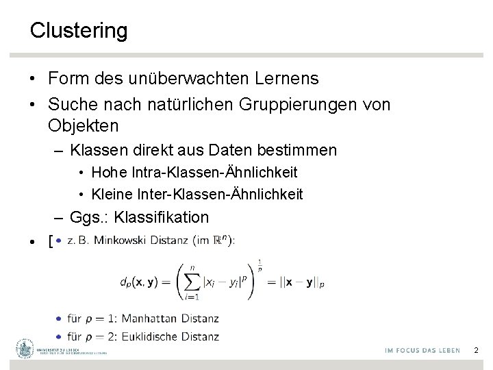
Clustering • Form des unüberwachten Lernens • Suche nach natürlichen Gruppierungen von Objekten – Klassen direkt aus Daten bestimmen • Hohe Intra-Klassen-Ähnlichkeit • Kleine Inter-Klassen-Ähnlichkeit – Ggs. : Klassifikation • Distanzmaße 2

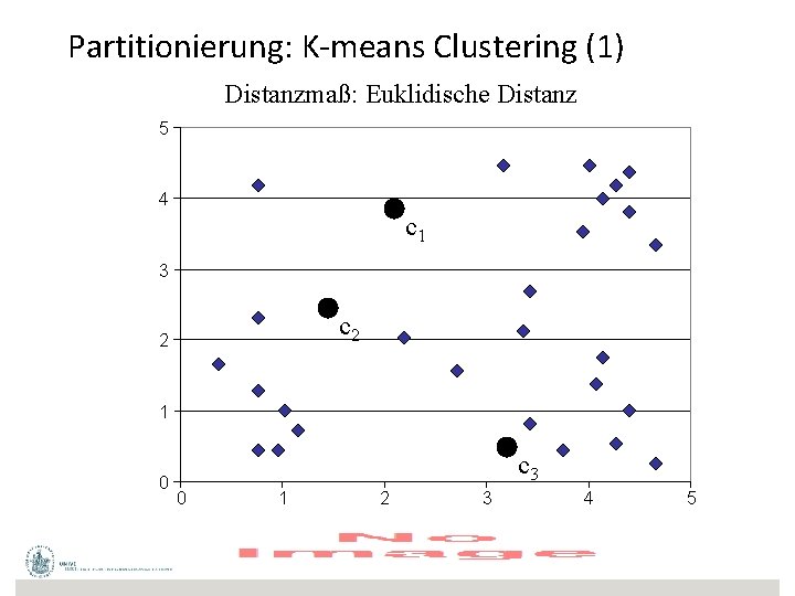
Partitionierung: K-means Clustering (1) Distanzmaß: Euklidische Distanz 5 4 c 1 3 c 2 2 1 0 c 3 0 1 2 3 4 5

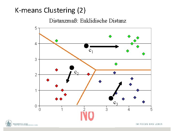
K-means Clustering (2) Distanzmaß: Euklidische Distanz 5 4 c 1 3 c 2 2 1 0 c 3 0 1 2 3 4 5

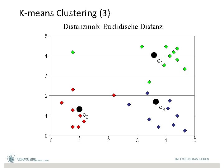
K-means Clustering (3) Distanzmaß: Euklidische Distanz 5 4 c 1 3 2 c 2 1 0 c 3 0 1 2 3 4 5

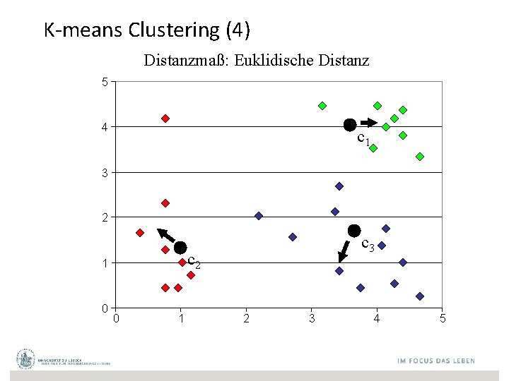
K-means Clustering (4) Distanzmaß: Euklidische Distanz 5 4 c 1 3 2 c 2 1 0 c 3 0 1 2 3 4 5

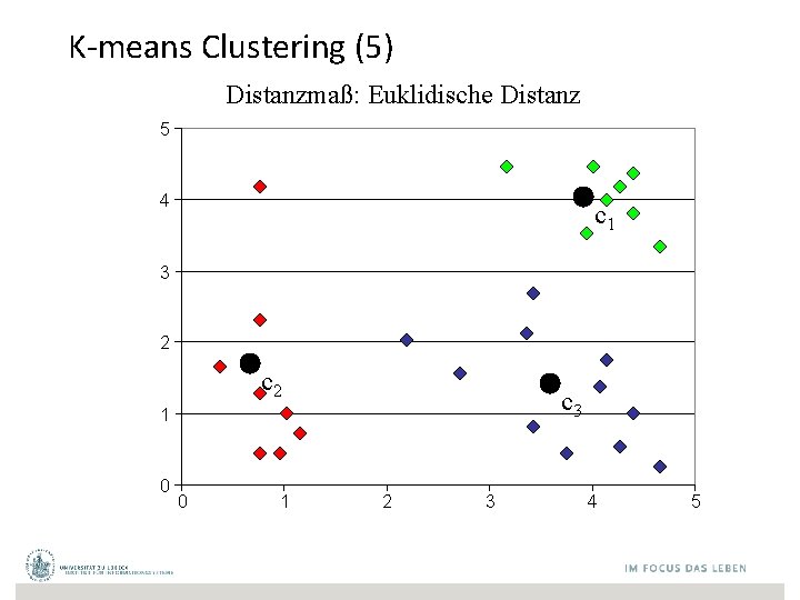
K-means Clustering (5) Distanzmaß: Euklidische Distanz 5 4 c 1 3 2 c 3 1 0 0 1 2 3 4 5

Acknowledgements This part is based on the following presentation: ANOVA: Analysis of Variation Math 243 Lecture R. Pruim (but contains changes and modifications)

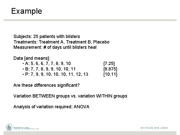
Example Subjects: 25 patients with blisters Treatments: Treatment A, Treatment B, Placebo Measurement: # of days until blisters heal Data [and means]: • A: 5, 6, 6, 7, 7, 8, 9, 10 • B: 7, 7, 8, 9, 9, 10, 11 • P: 7, 9, 9, 10, 10, 11, 12, 13 [7. 25] [8. 875] [10. 11] Are these differences significant? Variation BETWEEN groups vs. variation WITHIN groups Analysis of variation required: ANOVA

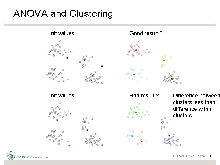
ANOVA and Clustering Init values Good result ? Init values Bad result ? Difference between clusters less than difference within clusters 10

The basic ANOVA situation Two variables: 1 Categorical (type, group), 1 Quantitative (value) Main Question: Do the (means of) the quantitative variables depend on the group (given by categorical variable) the individual is in? If categorical variable has only 2 values: • 2 -sample t-test ANOVA allows for 3 or more groups

What does ANOVA do? At its simplest (there are extensions) ANOVA tests the following hypotheses: H 0: The means of all the groups are equal. Ha: Not all the means are equal • doesn’t say how or which ones differ. • Can follow up with “multiple comparisons” Note: we usually refer to the sub-populations as “groups” when doing ANOVA.

Assumptions of ANOVA • Each group is approximately normal – Check this by looking at histograms or use assumptions – Can handle some non-normality, but not severe outliers • Standard deviations of each group are approximately equal – Rule of thumb: ratio of largest to smallest sample st. dev. must be less than 2: 1

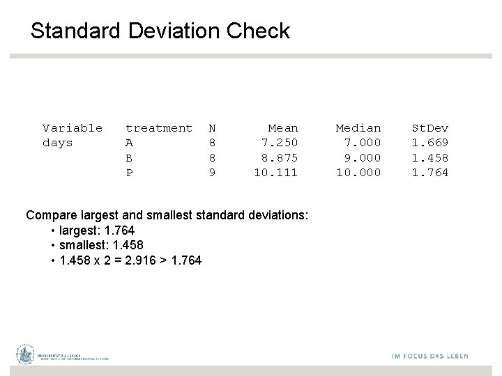
Standard Deviation Check Variable days treatment A B P N 8 8 9 Mean 7. 250 8. 875 10. 111 Compare largest and smallest standard deviations: • largest: 1. 764 • smallest: 1. 458 • 1. 458 x 2 = 2. 916 > 1. 764 Median 7. 000 9. 000 10. 000 St. Dev 1. 669 1. 458 1. 764

Notation for ANOVA • n = number of individuals all together • I = number of groups • = mean for entire data set Group i has • ni = # of individuals in group i • xij = value for individual j in group i • = mean for group i • si = standard deviation for group i

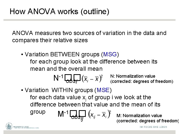
How ANOVA works (outline) ANOVA measures two sources of variation in the data and compares their relative sizes • Variation BETWEEN groups (MSG) for each group look at the difference between its mean and the overall mean N-1�� obsi N: Normalization value (corrected: degrees of freedom) • Variation WITHIN groups (MSE) for each data value xj of group i we look at the difference between that value and the mean of its group M-1�� M: Normalization value obsij (corrected: degrees of freedom)

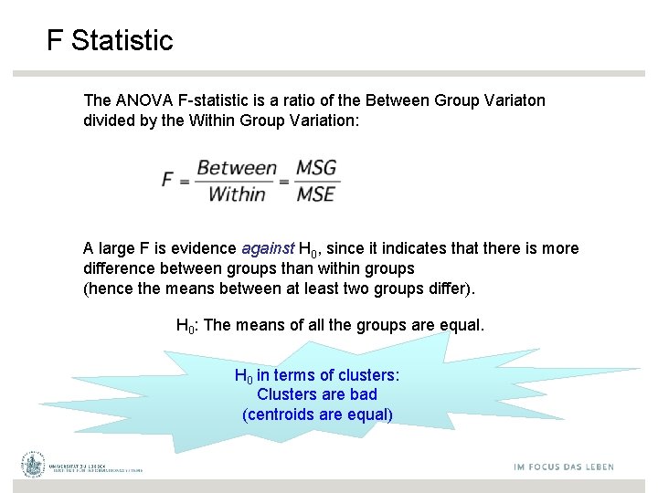
F Statistic The ANOVA F-statistic is a ratio of the Between Group Variaton divided by the Within Group Variation: A large F is evidence against H 0, since it indicates that there is more difference between groups than within groups (hence the means between at least two groups differ). H 0: The means of all the groups are equal. H 0 in terms of clusters: Clusters are bad (centroids are equal)

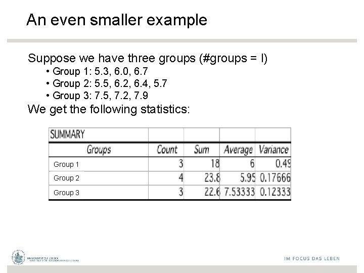
An even smaller example Suppose we have three groups (#groups = l) • Group 1: 5. 3, 6. 0, 6. 7 • Group 2: 5. 5, 6. 2, 6. 4, 5. 7 • Group 3: 7. 5, 7. 2, 7. 9 We get the following statistics: Group 1 Group 2 Group 3

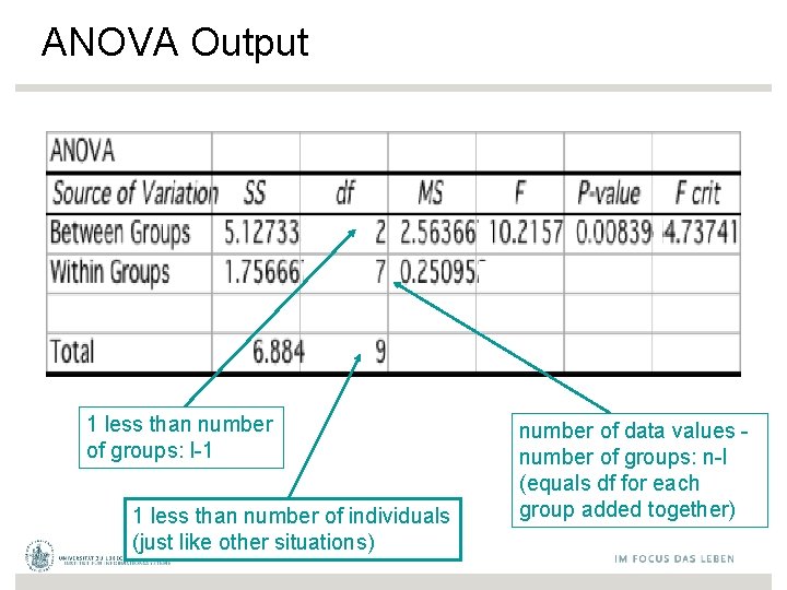
ANOVA Output 1 less than number of groups: l-1 1 less than number of individuals (just like other situations) number of data values - number of groups: n-l (equals df for each group added together)

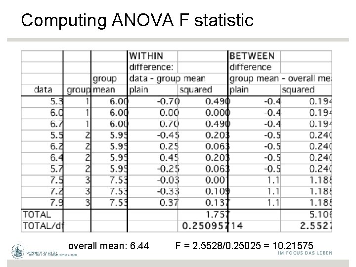
Computing ANOVA F statistic overall mean: 6. 44 F = 2. 5528/0. 25025 = 10. 21575

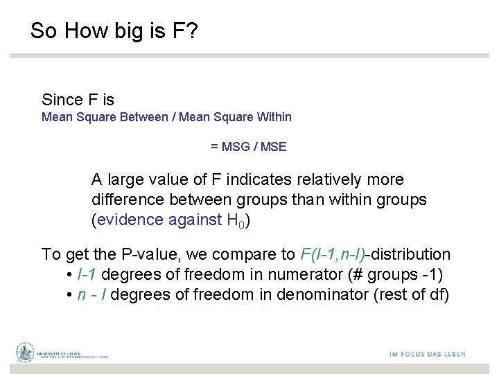
So How big is F? Since F is Mean Square Between / Mean Square Within = MSG / MSE A large value of F indicates relatively more difference between groups than within groups (evidence against H 0) To get the P-value, we compare to F(I-1, n-I)-distribution • I-1 degrees of freedom in numerator (# groups -1) • n - I degrees of freedom in denominator (rest of df)

F-Distribution 22

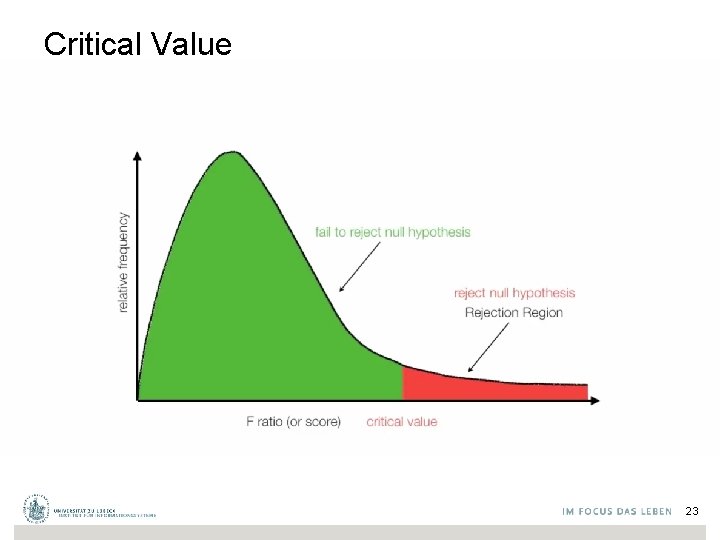
Critical Value 23

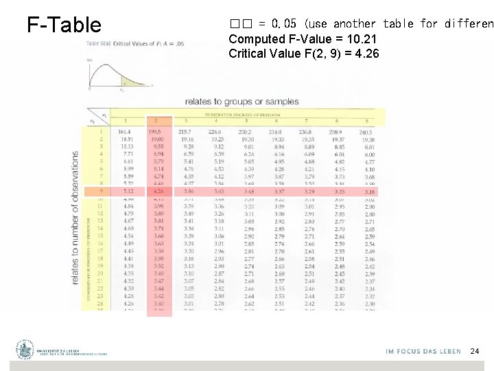
F-Table �� = 0. 05 (use another table for differen Computed F-Value = 10. 21 Critical Value F(2, 9) = 4. 26 24

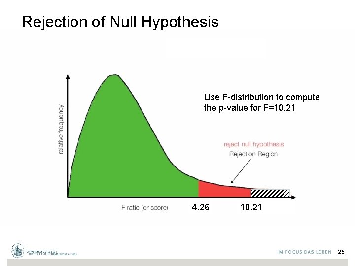
Rejection of Null Hypothesis Use F-distribution to compute the p-value for F=10. 21 4. 26 10. 21 25

Why not just do 3 pairwise t-tests? Answer: • At an error rate of 5% for each test (max pvalue), overall chance of type-I error is up to 1 -(. 95)3= 14% – If all 3 comparisons independent • For 6 groups: 6 C 2 = 15 pairwise t-tests; – High chance of finding something significant just by chance (if all tests were independent with a type-I error rate of 5% each) – Probability of at least one type-I error = 1 -(. 95)15=54%.

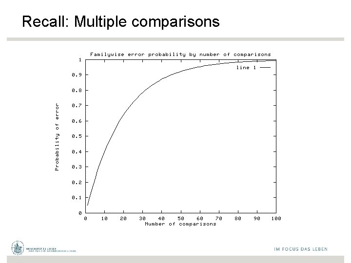
Recall: Multiple comparisons

Correction for multiple comparisons How to correct for multiple comparisons post-hoc… • Bonferroni correction (adjust �� by most conservative amount; assuming all tests independent, divide �� by the number of tests) • . . .

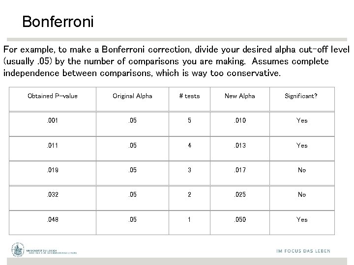
Bonferroni For example, to make a Bonferroni correction, divide your desired alpha cut-off level (usually. 05) by the number of comparisons you are making. Assumes complete independence between comparisons, which is way too conservative. Obtained P-value Original Alpha # tests New Alpha Significant? . 001 . 05 5 . 010 Yes . 011 . 05 4 . 013 Yes . 019 . 05 3 . 017 No . 032 . 05 2 . 025 No . 048 . 05 1 . 050 Yes

Multivariate Analysis of Variance: MANOVA • An extension of ANOVA in which main effects and interactions are assessed on a combination of DVs – IV = independent variable, manipulated variable (e. g. , Treatment) – DV = dependent variable, measured variable (e. g. , Mean) • MANOVA tests whether mean differences among groups on a combination of DVs is likely to occur by chance • New DVs are created that are linear combinations of the individual DVs such that the difference between groups is maximized • The questions are mostly the same as ANOVA just on the linearly combined DVs instead just one DV

Are there any interactions among the IVs? • Does change in the linearly combined DV for one IV depend on the levels of another IV? • For example: Given three types of treatment, does one treatment work better for men and another work better for women?

Basic Requirements • 2 or more DVs (Interval, Ratio) • 1 or more categorical IVs (Nominal, Ordinal)

MANOVA advantages over ANOVA • By measuring multiple DVs you increase your chances for finding a group difference • With a single DV you “put all of your eggs in one basket” • Multiple measures usually do not “cost” a great deal more and you are more likely to find a difference on at least one

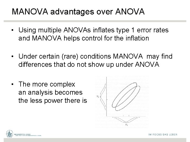
MANOVA advantages over ANOVA • Using multiple ANOVAs inflates type 1 error rates and MANOVA helps control for the inflation • Under certain (rare) conditions MANOVA may find differences that do not show up under ANOVA • The more complex an analysis becomes the less power there is

MANOVA • A new DV is created that is a linear combination of the individual DVs that maximizes the difference between groups. • In factorial designs a different linear combination of the DVs is created for each main effect and interaction that maximizes the group difference separately. • Also when the IVs have more than one level the DVs can be recombined to maximize paired comparisons

Discriminant Function Analysis • Used to predict group membership from a set of continuous predictors • Think of it as MANOVA in reverse – in MANOVA we asked if groups are significantly different on a set of linearly combined DVs. If this is true, than those same “DVs” can be used to predict group membership. • How can continuous variables be linearly combined to best classify a subject into a group? 36

Basics • MANOVA and disriminant function analysis are mathematically identical but are different in terms of emphasis – – discrim is usually concerned with actually putting people into groups (classification) and testing how well (or how poorly) subjects are classified Essentially, discrim is interested in exactly how the groups are differentiated not just that they are significantly different (as in MANOVA)

Questions • • the primary goal is to find a dimension(s) that groups differ on and create classification functions Can group membership be accurately predicted by a set of predictors? – Essentially the same question as MANOVA