Econometrics 2 Lecture 4 Lag Structures Cointegration Contents

Econometrics 2 - Lecture 4 Lag Structures, Cointegration

Contents n n n n n Dynamic Models Lag Structure: Estimation ADL Models for Expectations Models with Non-stationary Variables Cointegration Test for Cointegration Error-correction Model April 5, 2013 Hackl, Econometrics 2, Lecture 4 2

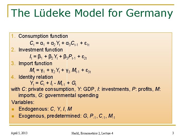
The Lüdeke Model for Germany 1. Consumption function Ct = α 1 + α 2 Yt + α 3 Ct-1 + ε 1 t 2. Investment function It = β 1 + β 2 Yt + β 3 Pt-1 + ε 2 t 3. Import function Mt = γ 1 + γ 2 Yt + γ 3 Mt-1 + ε 3 t 4. Identity relation Yt = Ct + It - Mt-1 + Gt with C: private consumption, Y: GDP, I: investments, P: profits, M: imports, G: governmental spending Variables: n Endogenous: C, Y, I, M n Exogenous, predetermined: G, P-1, C-1, M-1 April 5, 2013 Hackl, Econometrics 2, Lecture 4 3

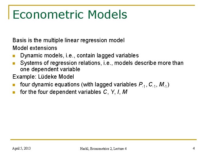
Econometric Models Basis is the multiple linear regression model Model extensions n Dynamic models, i. e. , contain lagged variables n Systems of regression relations, i. e. , models describe more than one dependent variable Example: Lüdeke Model n four dynamic equations (with lagged variables P-1, C-1, M-1) n for the four dependent variables C, Y, I, M April 5, 2013 Hackl, Econometrics 2, Lecture 4 4

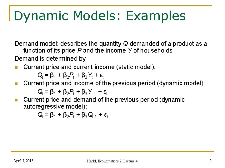
Dynamic Models: Examples Demand model: describes the quantity Q demanded of a product as a function of its price P and the income Y of households Demand is determined by n Current price and current income (static model): Qt = β 1 + β 2 Pt + β 3 Yt + εt n Current price and income of the previous period (dynamic model): Qt = β 1 + β 2 Pt + β 3 Yt-1 + εt n Current price and demand of the previous period (dynamic autoregressive model): Qt = β 1 + β 2 Pt + β 3 Qt-1 + εt April 5, 2013 Hackl, Econometrics 2, Lecture 4 5

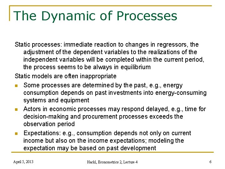
The Dynamic of Processes Static processes: immediate reaction to changes in regressors, the adjustment of the dependent variables to the realizations of the independent variables will be completed within the current period, the process seems to be always in equilibrium Static models are often inappropriate n Some processes are determined by the past, e. g. , energy consumption depends on past investments into energy-consuming systems and equipment n Actors in economic processes may respond delayed, e. g. , time for decision-making and procurement processes exceeds the observation period n Expectations: e. g. , consumption depends not only on current income but also on the income expectations; modeling the expectation may be based on past development April 5, 2013 Hackl, Econometrics 2, Lecture 4 6

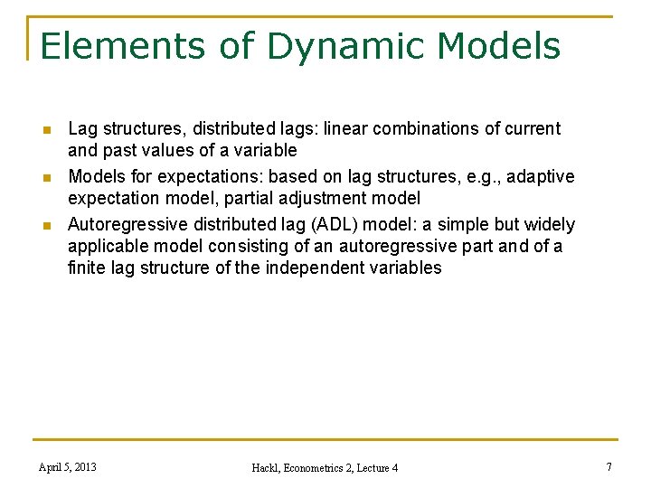
Elements of Dynamic Models n n n Lag structures, distributed lags: linear combinations of current and past values of a variable Models for expectations: based on lag structures, e. g. , adaptive expectation model, partial adjustment model Autoregressive distributed lag (ADL) model: a simple but widely applicable model consisting of an autoregressive part and of a finite lag structure of the independent variables April 5, 2013 Hackl, Econometrics 2, Lecture 4 7

Contents n n n n n Dynamic Models Lag Structure: Estimation ADL Models for Expectations Models with Non-stationary Variables Cointegration Test for Cointegration Error-correction Model April 5, 2013 Hackl, Econometrics 2, Lecture 4 8

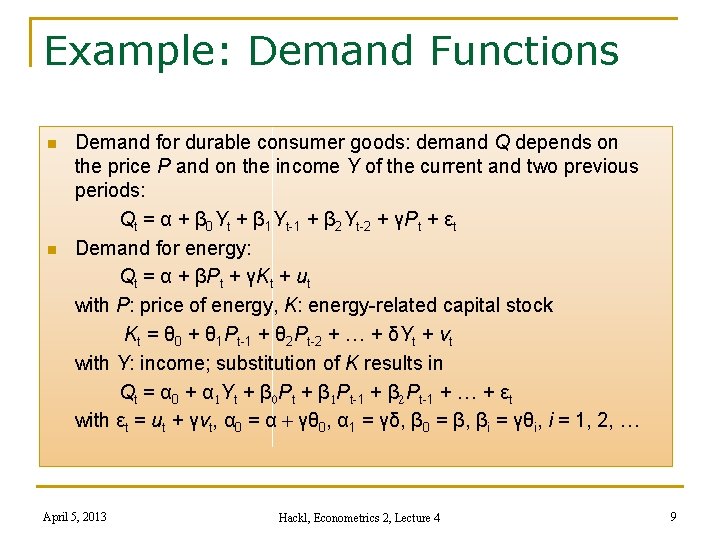
Example: Demand Functions n n Demand for durable consumer goods: demand Q depends on the price P and on the income Y of the current and two previous periods: Qt = α + β 0 Yt + β 1 Yt-1 + β 2 Yt-2 + γPt + εt Demand for energy: Qt = α + βPt + γKt + ut with P: price of energy, K: energy-related capital stock Kt = θ 0 + θ 1 Pt-1 + θ 2 Pt-2 + … + δYt + vt with Y: income; substitution of K results in Qt = α 0 + α 1 Yt + β 0 Pt + β 1 Pt-1 + β 2 Pt-1 + … + εt with εt = ut + γvt, α 0 = α + γθ 0, α 1 = γδ, β 0 = β, βi = γθi, i = 1, 2, … April 5, 2013 Hackl, Econometrics 2, Lecture 4 9

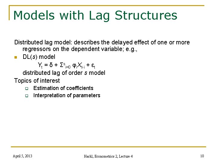
Models with Lag Structures Distributed lag model: describes the delayed effect of one or more regressors on the dependent variable; e. g. , n DL(s) model Yt = δ + Σsi=0 φi. Xt-i + εt distributed lag of order s model Topics of interest q q April 5, 2013 Estimation of coefficients Interpretation of parameters Hackl, Econometrics 2, Lecture 4 10

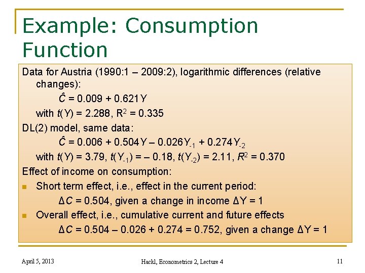
Example: Consumption Function Data for Austria (1990: 1 – 2009: 2), logarithmic differences (relative changes): Ĉ = 0. 009 + 0. 621 Y with t(Y) = 2. 288, R 2 = 0. 335 DL(2) model, same data: Ĉ = 0. 006 + 0. 504 Y – 0. 026 Y-1 + 0. 274 Y-2 with t(Y) = 3. 79, t(Y-1) = – 0. 18, t(Y-2) = 2. 11, R 2 = 0. 370 Effect of income on consumption: n Short term effect, i. e. , effect in the current period: ΔC = 0. 504, given a change in income ΔY = 1 n Overall effect, i. e. , cumulative current and future effects ΔC = 0. 504 – 0. 026 + 0. 274 = 0. 752, given a change ΔY = 1 April 5, 2013 Hackl, Econometrics 2, Lecture 4 11

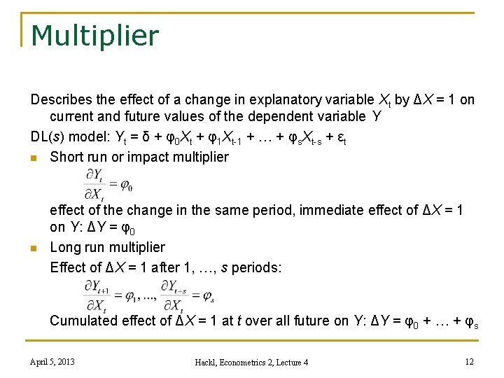
Multiplier Describes the effect of a change in explanatory variable Xt by ΔX = 1 on current and future values of the dependent variable Y DL(s) model: Yt = δ + φ0 Xt + φ1 Xt-1 + … + φs. Xt-s + εt n Short run or impact multiplier n effect of the change in the same period, immediate effect of ΔX = 1 on Y: ΔY = φ0 Long run multiplier Effect of ΔX = 1 after 1, …, s periods: Cumulated effect of ΔX = 1 at t over all future on Y: ΔY = φ0 + … + φs April 5, 2013 Hackl, Econometrics 2, Lecture 4 12

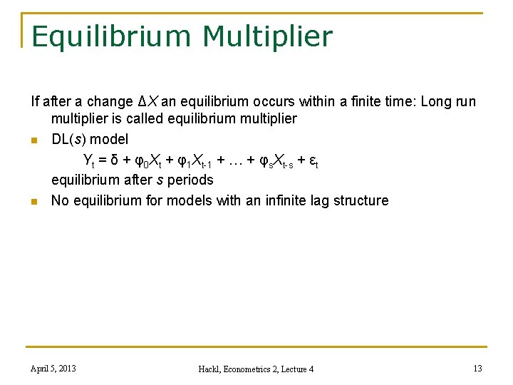
Equilibrium Multiplier If after a change ΔX an equilibrium occurs within a finite time: Long run multiplier is called equilibrium multiplier n DL(s) model Yt = δ + φ0 Xt + φ1 Xt-1 + … + φs. Xt-s + εt equilibrium after s periods n No equilibrium for models with an infinite lag structure April 5, 2013 Hackl, Econometrics 2, Lecture 4 13

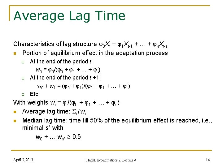
Average Lag Time Characteristics of lag structure φ0 Xt + φ1 Xt-1 + … + φs. Xt-s n Portion of equilibrium effect in the adaptation process q q q At the end of the period t: w 0 = φ0/(φ0 + φ1 + … + φs) At the end of the period t +1: w 0 + w 1 = (φ0 + φ1)/(φ0 + φ1 + … + φs) Etc. With weights wi = φi/(φ0 + φ1 + … + φs) n Average lag time: Si i wi n Median lag time: time till 50% of the equilibrium effect is reached, i. e. , minimal s* with w 0 + … ws* ≥ 0. 5 April 5, 2013 Hackl, Econometrics 2, Lecture 4 14

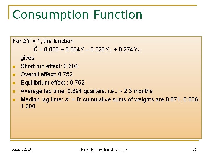
Consumption Function For ΔY = 1, the function Ĉ = 0. 006 + 0. 504 Y – 0. 026 Y-1 + 0. 274 Y-2 gives n Short run effect: 0. 504 n Overall effect: 0. 752 n Equilibrium effect : 0. 752 n Average lag time: 0. 694 quarters, i. e. , ~ 2. 3 months n Median lag time: s* = 0; cumulative sums of weights are 0. 671, 0. 636, 1. 000 April 5, 2013 Hackl, Econometrics 2, Lecture 4 15

Contents n n n n n Dynamic Models Lag Structure: Estimation ADL Models for Expectations Models with Non-stationary Variables Cointegration Test for Cointegration Error-correction Model April 5, 2013 Hackl, Econometrics 2, Lecture 4 16

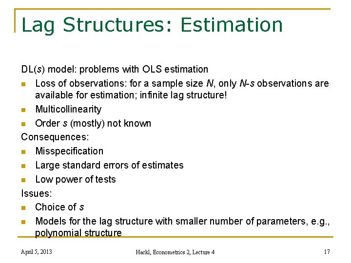
Lag Structures: Estimation DL(s) model: problems with OLS estimation n Loss of observations: for a sample size N, only N-s observations are available for estimation; infinite lag structure! n Multicollinearity n Order s (mostly) not known Consequences: n Misspecification n Large standard errors of estimates n Low power of tests Issues: n Choice of s n Models for the lag structure with smaller number of parameters, e. g. , polynomial structure April 5, 2013 Hackl, Econometrics 2, Lecture 4 17

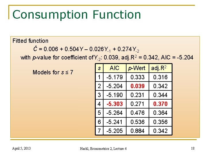
Consumption Function Fitted function Ĉ = 0. 006 + 0. 504 Y – 0. 026 Y-1 + 0. 274 Y-2 with p-value for coefficient of. Y-2: 0. 039, adj. R 2 = 0. 342, AIC = -5. 204 s AIC p-Wert adj. R 2 Models for s ≤ 7 1 -5. 179 0. 333 0. 316 April 5, 2013 2 -5. 204 0. 039 0. 342 3 -5. 190 0. 231 0. 344 4 -5. 303 0. 271 0. 370 5 -5. 264 0. 476 0. 364 6 -5. 241 0. 536 0. 356 7 -5. 205 0. 884 0. 342 Hackl, Econometrics 2, Lecture 4 18

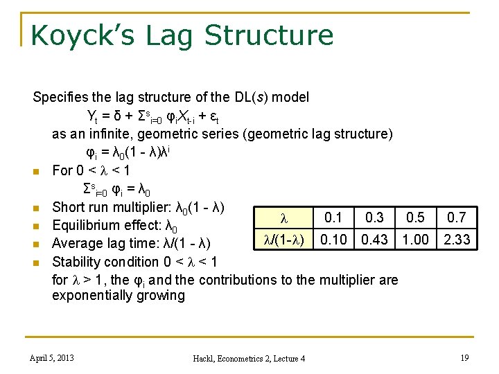
Koyck’s Lag Structure Specifies the lag structure of the DL(s) model Yt = δ + Σsi=0 φi. Xt-i + εt as an infinite, geometric series (geometric lag structure) φi = λ 0(1 - λ)λi n For 0 < l < 1 Σsi=0 φi = λ 0 n Short run multiplier: λ 0(1 - λ) 0. 1 0. 3 0. 5 l n Equilibrium effect: λ 0 l/(1 -l) 0. 10 0. 43 1. 00 n Average lag time: λ/(1 - λ) n Stability condition 0 < l < 1 for l > 1, the φi and the contributions to the multiplier are exponentially growing April 5, 2013 Hackl, Econometrics 2, Lecture 4 0. 7 2. 33 19

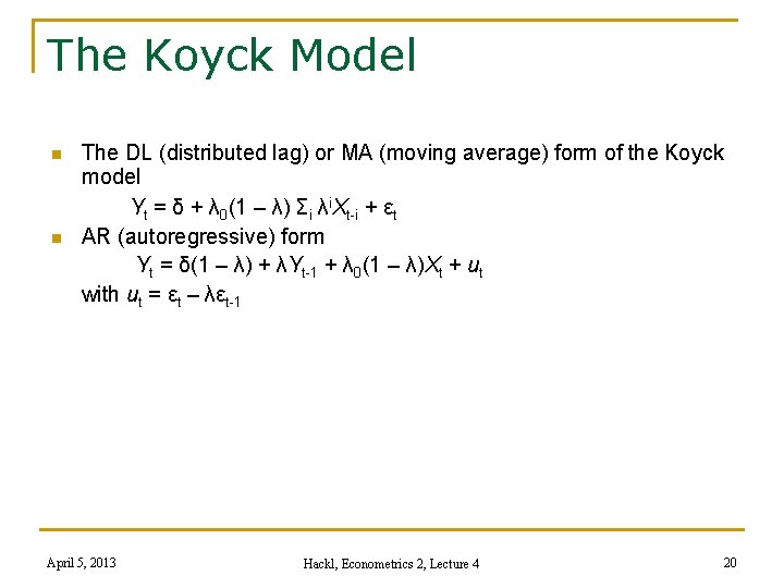
The Koyck Model n n The DL (distributed lag) or MA (moving average) form of the Koyck model Yt = δ + λ 0(1 – λ) Σi λi. Xt-i + εt AR (autoregressive) form Yt = δ(1 – λ) + λYt-1 + λ 0(1 – λ)Xt + ut with ut = εt – λεt-1 April 5, 2013 Hackl, Econometrics 2, Lecture 4 20

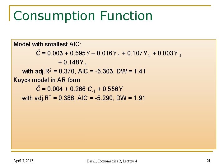
Consumption Function Model with smallest AIC: Ĉ = 0. 003 + 0. 595 Y – 0. 016 Y-1 + 0. 107 Y-2 + 0. 003 Y-3 + 0. 148 Y-4 with adj. R 2 = 0. 370, AIC = -5. 303, DW = 1. 41 Koyck model in AR form Ĉ = 0. 004 + 0. 286 C-1 + 0. 556 Y with adj. R 2 = 0. 388, AIC = -5. 290, DW = 1. 91 April 5, 2013 Hackl, Econometrics 2, Lecture 4 21

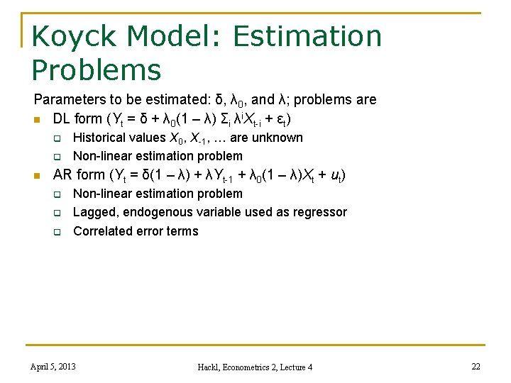
Koyck Model: Estimation Problems Parameters to be estimated: δ, λ 0, and λ; problems are n DL form (Yt = δ + λ 0(1 – λ) Σi λi. Xt-i + εt) q q n Historical values X 0, X-1, … are unknown Non-linear estimation problem AR form (Yt = δ(1 – λ) + λYt-1 + λ 0(1 – λ)Xt + ut) q q q Non-linear estimation problem Lagged, endogenous variable used as regressor Correlated error terms April 5, 2013 Hackl, Econometrics 2, Lecture 4 22

Contents n n n n n Dynamic Models Lag Structure: Estimation ADL Models for Expectations Models with Non-stationary Variables Cointegration Test for Cointegration Error-correction Model April 5, 2013 Hackl, Econometrics 2, Lecture 4 23

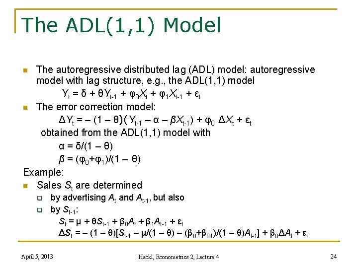
The ADL(1, 1) Model The autoregressive distributed lag (ADL) model: autoregressive model with lag structure, e. g. , the ADL(1, 1) model Yt = δ + θYt-1 + φ0 Xt + φ1 Xt-1 + εt n The error correction model: ΔYt = – (1 – θ)(Yt-1 – α – βXt-1) + φ0 ΔXt + εt obtained from the ADL(1, 1) model with α = δ/(1 – θ) β = (φ0+φ1)/(1 – θ) Example: n Sales St are determined n q q by advertising At and At-1, but also by St-1: St = μ + θSt-1 + β 0 At + β 1 At-1 + εt ΔSt = – (1 – θ)[St-1 – μ/(1 – θ) – (β 0+β 01)/(1 – θ)At-1] + β 0ΔAt + εt April 5, 2013 Hackl, Econometrics 2, Lecture 4 24

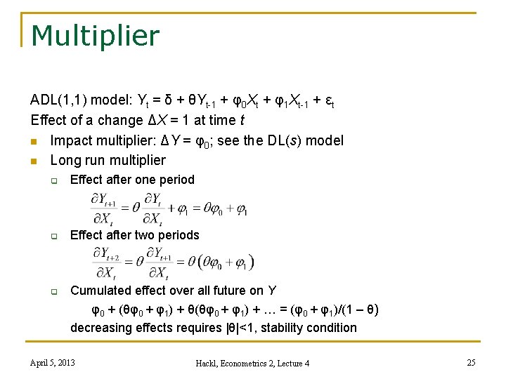
Multiplier ADL(1, 1) model: Yt = δ + θYt-1 + φ0 Xt + φ1 Xt-1 + εt Effect of a change ΔX = 1 at time t n Impact multiplier: ΔY = φ0; see the DL(s) model n Long run multiplier q Effect after one period q Effect after two periods q Cumulated effect over all future on Y φ0 + (θφ0 + φ1) + θ(θφ0 + φ1) + … = (φ0 + φ1)/(1 – θ) decreasing effects requires |θ|<1, stability condition April 5, 2013 Hackl, Econometrics 2, Lecture 4 25

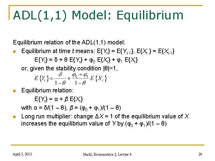
ADL(1, 1) Model: Equilibrium relation of the ADL(1, 1) model: n Equilibrium at time t means: E{Yt} = E{Yt-1}, E{Xt } = E{Xt-1} E{Yt} = δ + θ E{Yt} + φ0 E{Xt} + φ1 E{Xt} or, given the stability condition |θ|<1, n n Equilibrium relation: E{Yt} = α + β E{Xt} with α = δ/(1 – θ), β = (φ0 + φ1)/(1 – θ) Long run multiplier: change ΔX = 1 of the equilibrium value of X increases the equilibrium value of Y by (φ0 + φ1)/(1 – θ) April 5, 2013 Hackl, Econometrics 2, Lecture 4 26

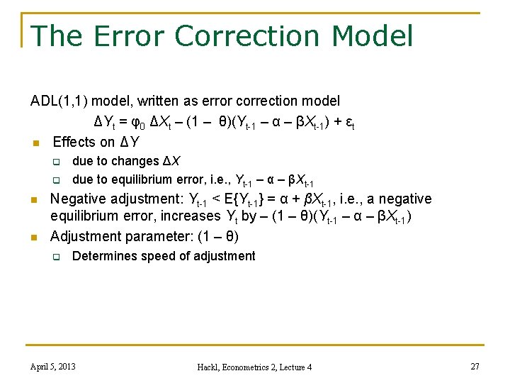
The Error Correction Model ADL(1, 1) model, written as error correction model ΔYt = φ0 ΔXt – (1 – θ)(Yt-1 – α – βXt-1) + εt n Effects on ΔY q q n n due to changes ΔX due to equilibrium error, i. e. , Yt-1 – α – βXt-1 Negative adjustment: Yt-1 < E{Yt-1} = α + βXt-1, i. e. , a negative equilibrium error, increases Yt by – (1 – θ)(Yt-1 – α – βXt-1) Adjustment parameter: (1 – θ) q Determines speed of adjustment April 5, 2013 Hackl, Econometrics 2, Lecture 4 27

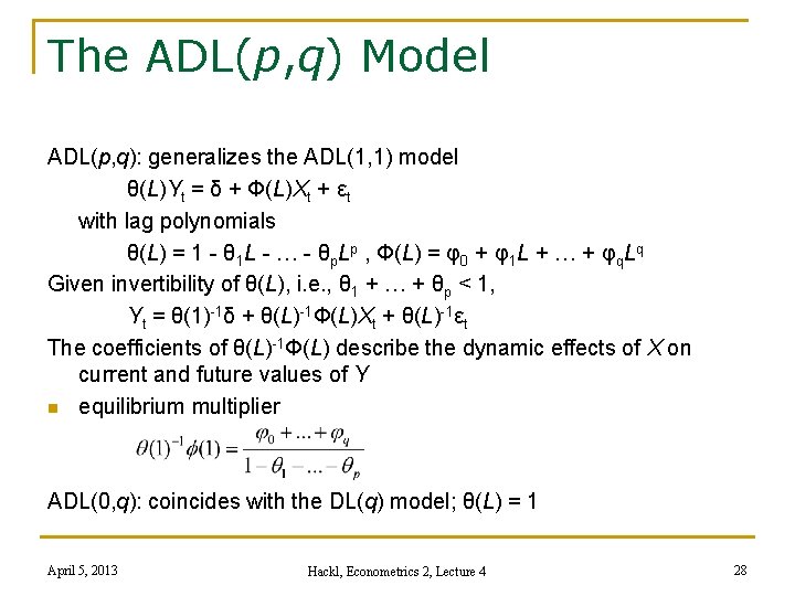
The ADL(p, q) Model ADL(p, q): generalizes the ADL(1, 1) model θ(L)Yt = δ + Φ(L)Xt + εt with lag polynomials θ(L) = 1 - θ 1 L - … - θp. Lp , Φ(L) = φ0 + φ1 L + … + φq. Lq Given invertibility of θ(L), i. e. , θ 1 + … + θp < 1, Yt = θ(1)-1δ + θ(L)-1Φ(L)Xt + θ(L)-1εt The coefficients of θ(L)-1Φ(L) describe the dynamic effects of X on current and future values of Y n equilibrium multiplier ADL(0, q): coincides with the DL(q) model; θ(L) = 1 April 5, 2013 Hackl, Econometrics 2, Lecture 4 28

ADL Model: Estimation ADL(p, q) model n error terms εt: white noise, independent of Xt, …, Xt-q and Yt-1, …, Xt-p OLS estimators are consistent April 5, 2013 Hackl, Econometrics 2, Lecture 4 29

Contents n n n n n Dynamic Models Lag Structure: Estimation ADL Models for Expectations Models with Non-stationary Variables Cointegration Test for Cointegration Error-correction Model April 5, 2013 Hackl, Econometrics 2, Lecture 4 30

Expectations in Economic Processes Expectations play important role in economic processes Examples: n Consumption depends not only on current income but also on the income expectations; modeling the expectation may be based on past development n Investments depend upon expected profits n Interest rates depend upon expected development of the financial market n Etc. Expectations n cannot be observed, but n can be modeled using assumptions on the mechanism of adapting expectations April 5, 2013 Hackl, Econometrics 2, Lecture 4 31

Models for Adapting Expectations Naive model of adapting expectations: the (for the next period) expected value equals the actual value n Model of adaptive expectation n Partial adjustment model The latter two models are based on Koyck’s lag structure n April 5, 2013 Hackl, Econometrics 2, Lecture 4 32

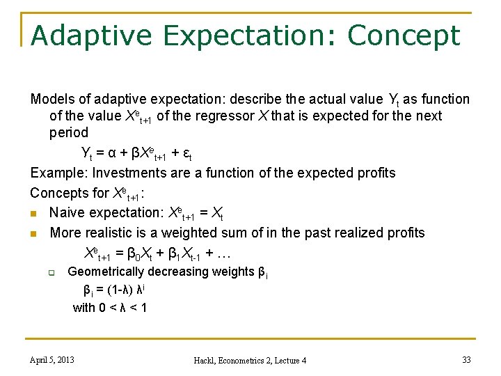
Adaptive Expectation: Concept Models of adaptive expectation: describe the actual value Yt as function of the value Xet+1 of the regressor X that is expected for the next period Yt = α + βXet+1 + εt Example: Investments are a function of the expected profits Concepts for Xet+1: n Naive expectation: Xet+1 = Xt n More realistic is a weighted sum of in the past realized profits Xet+1 = β 0 Xt + β 1 Xt-1 + … Geometrically decreasing weights βi βi = (1 -λ) λi with 0 < λ < 1 q April 5, 2013 Hackl, Econometrics 2, Lecture 4 33

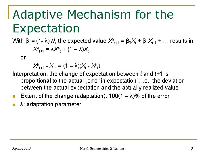
Adaptive Mechanism for the Expectation With βi = (1 - λ) λi, the expected value Xet+1 = β 0 Xt + β 1 Xt-1 + … results in Xet+1 = λXet + (1 – λ)Xt or Xet+1 - Xet = (1 – λ)(Xt - Xet) Interpretation: the change of expectation between t and t+1 is proportional to the actual „error in expectation”, i. e. , the deviation between the actual expectation and the actually realized value n Extent of the change (adaptation): 100(1 – λ)% of the error n λ: adaptation parameter April 5, 2013 Hackl, Econometrics 2, Lecture 4 34

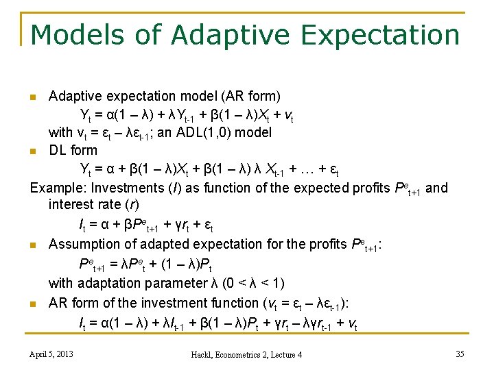
Models of Adaptive Expectation Adaptive expectation model (AR form) Yt = α(1 – λ) + λYt-1 + β(1 – λ)Xt + vt with vt = εt – λεt-1; an ADL(1, 0) model n DL form Yt = α + β(1 – λ)Xt + β(1 – λ) λ Xt-1 + … + εt Example: Investments (I) as function of the expected profits Pet+1 and interest rate (r) It = α + βPet+1 + γrt + εt n Assumption of adapted expectation for the profits Pet+1: Pet+1 = λPet + (1 – λ)Pt with adaptation parameter λ (0 < λ < 1) n AR form of the investment function (vt = εt – λεt-1): It = α(1 – λ) + λIt-1 + β(1 – λ)Pt + γrt – λγrt-1 + vt n April 5, 2013 Hackl, Econometrics 2, Lecture 4 35

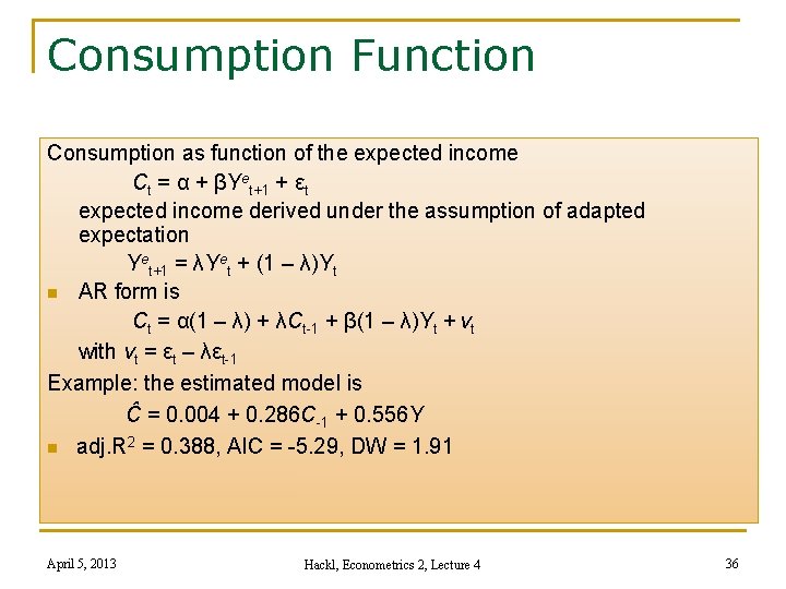
Consumption Function Consumption as function of the expected income Ct = α + βYet+1 + εt expected income derived under the assumption of adapted expectation Yet+1 = λYet + (1 – λ)Yt n AR form is Ct = α(1 – λ) + λCt-1 + β(1 – λ)Yt + vt with vt = εt – λεt-1 Example: the estimated model is Ĉ = 0. 004 + 0. 286 C-1 + 0. 556 Y n adj. R 2 = 0. 388, AIC = -5. 29, DW = 1. 91 April 5, 2013 Hackl, Econometrics 2, Lecture 4 36

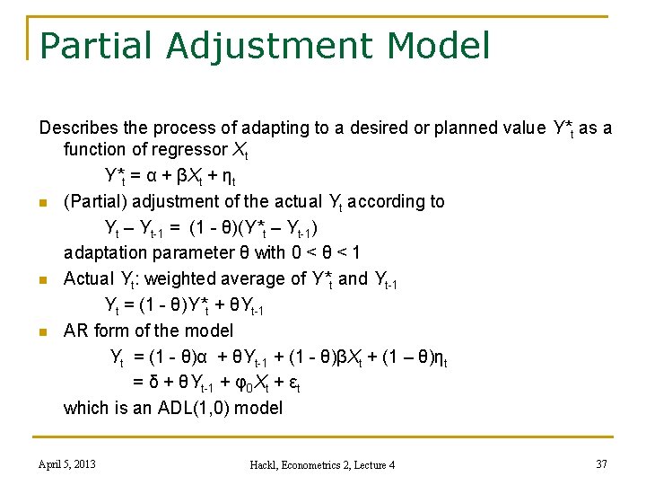
Partial Adjustment Model Describes the process of adapting to a desired or planned value Y*t as a function of regressor Xt Y*t = α + βXt + ηt n (Partial) adjustment of the actual Yt according to Yt – Yt-1 = (1 - θ)(Y*t – Yt-1) adaptation parameter θ with 0 < θ < 1 n Actual Yt: weighted average of Y*t and Yt-1 Yt = (1 - θ)Y*t + θYt-1 n AR form of the model Yt = (1 - θ)α + θYt-1 + (1 - θ)βXt + (1 – θ)ηt = δ + θYt-1 + φ0 Xt + εt which is an ADL(1, 0) model April 5, 2013 Hackl, Econometrics 2, Lecture 4 37

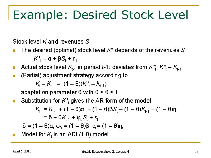
Example: Desired Stock Level Stock level K and revenues S n The desired (optimal) stock level K* depends of the revenues S K*t = α + βSt + ηt n Actual stock level Kt-1 in period t-1: deviates from K*t: K*t – Kt-1 n (Partial) adjustment strategy according to Kt – Kt-1 = (1 – θ)(K*t – Kt-1) adaptation parameter θ with 0 < θ < 1 n Substitution for K*t gives the AR form of the model Kt = Kt-1 + (1 – θ)α + (1 – θ)βSt – (1 – θ)Kt-1 + (1 – θ)ηt = δ + θKt-1 + φ0 St + εt δ = (1 – θ)α, φ0 = (1 – θ)β, εt = (1 – θ)ηt n Model for Kt is an ADL(1, 0) model April 5, 2013 Hackl, Econometrics 2, Lecture 4 38

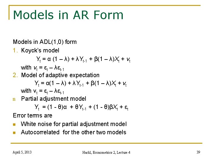
Models in AR Form Models in ADL(1, 0) form 1. Koyck’s model Yt = α (1 – λ) + λYt-1 + β(1 – λ)Xt + vt with vt = εt – λεt-1 2. Model of adaptive expectation Yt = α(1 – λ) + λYt-1 + β(1 – λ)Xt + vt with vt = εt – λεt-1 n Partial adjustment model Yt = (1 - θ)α + θYt-1 + (1 - θ)βXt + εt Error terms are n White noise for partial adjustment model n Autocorrelated for the other two models April 5, 2013 Hackl, Econometrics 2, Lecture 4 39

Contents n n n n n Dynamic Models Lag Structure: Estimation ADL Models for Expectations Models with Non-stationary Variables Cointegration Test for Cointegration Error-correction Model April 5, 2013 Hackl, Econometrics 2, Lecture 4 40

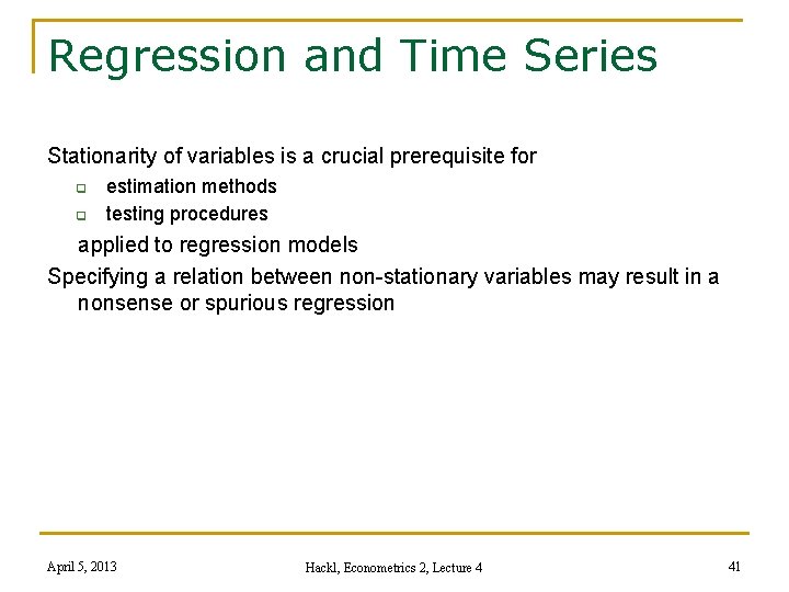
Regression and Time Series Stationarity of variables is a crucial prerequisite for q q estimation methods testing procedures applied to regression models Specifying a relation between non-stationary variables may result in a nonsense or spurious regression April 5, 2013 Hackl, Econometrics 2, Lecture 4 41

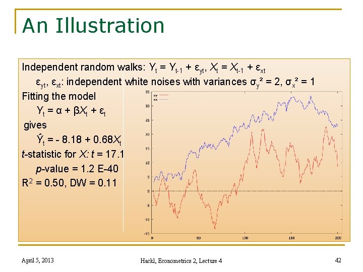
An Illustration Independent random walks: Yt = Yt-1 + εyt, Xt = Xt-1 + εxt εyt, εxt: independent white noises with variances σy² = 2, σx² = 1 Fitting the model Yt = α + βXt + εt gives Ŷt = - 8. 18 + 0. 68 Xt t-statistic for X: t = 17. 1 p-value = 1. 2 E-40 R 2 = 0. 50, DW = 0. 11 April 5, 2013 Hackl, Econometrics 2, Lecture 4 42

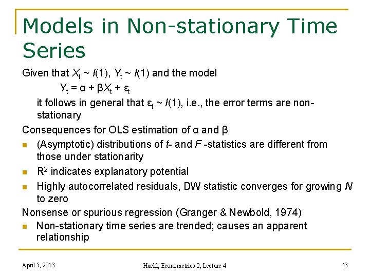
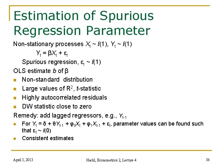
Models in Non-stationary Time Series Given that Xt ~ I(1), Yt ~ I(1) and the model Yt = α + βXt + εt it follows in general that εt ~ I(1), i. e. , the error terms are non- stationary Consequences for OLS estimation of α and β n (Asymptotic) distributions of t- and F -statistics are different from those under stationarity n R 2 indicates explanatory potential n Highly autocorrelated residuals, DW statistic converges for growing N to zero Nonsense or spurious regression (Granger & Newbold, 1974) n Non-stationary time series are trended; causes an apparent relationship April 5, 2013 Hackl, Econometrics 2, Lecture 4 43

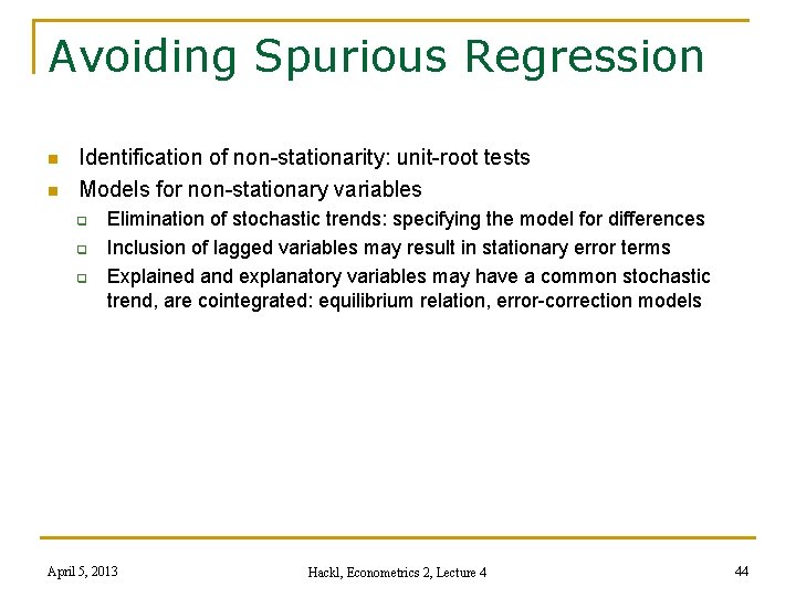
Avoiding Spurious Regression n n Identification of non-stationarity: unit-root tests Models for non-stationary variables q q q Elimination of stochastic trends: specifying the model for differences Inclusion of lagged variables may result in stationary error terms Explained and explanatory variables may have a common stochastic trend, are cointegrated: equilibrium relation, error-correction models April 5, 2013 Hackl, Econometrics 2, Lecture 4 44

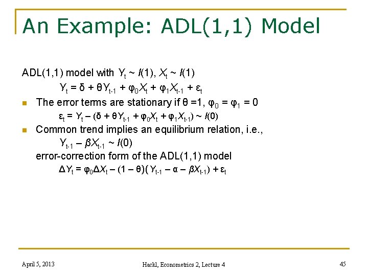
An Example: ADL(1, 1) Model ADL(1, 1) model with Yt ~ I(1), Xt ~ I(1) Yt = δ + θYt-1 + φ0 Xt + φ1 Xt-1 + εt n The error terms are stationary if θ =1, φ0 = φ1 = 0 εt = Yt – (δ + θYt-1 + φ0 Xt + φ1 Xt-1) ~ I(0) n Common trend implies an equilibrium relation, i. e. , Yt-1 – βXt-1 ~ I(0) error-correction form of the ADL(1, 1) model ΔYt = φ0ΔXt – (1 – θ)(Yt-1 – α – βXt-1) + εt April 5, 2013 Hackl, Econometrics 2, Lecture 4 45

Contents n n n n n Dynamic Models Lag Structure: Estimation ADL Models for Expectations Models with Non-stationary Variables Cointegration Test for Cointegration Error-correction Model April 5, 2013 Hackl, Econometrics 2, Lecture 4 46

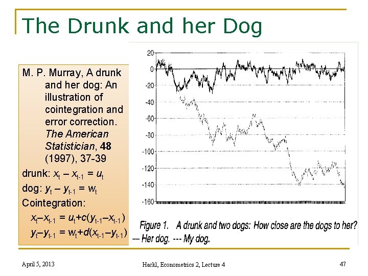
The Drunk and her Dog M. P. Murray, A drunk and her dog: An illustration of cointegration and error correction. The American Statistician, 48 (1997), 37 -39 drunk: xt – xt-1 = ut dog: yt – yt-1 = wt Cointegration: xt–xt-1 = ut+c(yt-1–xt-1) yt–yt-1 = wt+d(xt-1–yt-1) April 5, 2013 Hackl, Econometrics 2, Lecture 4 47

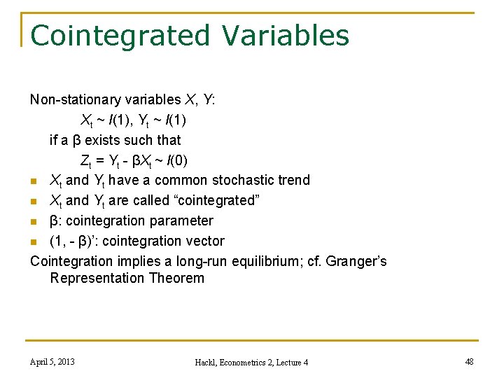
Cointegrated Variables Non-stationary variables X, Y: Xt ~ I(1), Yt ~ I(1) if a β exists such that Zt = Yt - βXt ~ I(0) n Xt and Yt have a common stochastic trend n Xt and Yt are called “cointegrated” n β: cointegration parameter n (1, - β)’: cointegration vector Cointegration implies a long-run equilibrium; cf. Granger’s Representation Theorem April 5, 2013 Hackl, Econometrics 2, Lecture 4 48

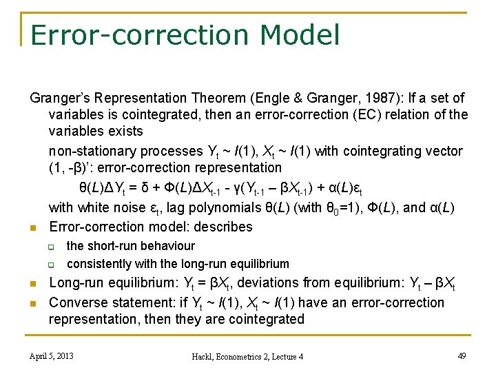
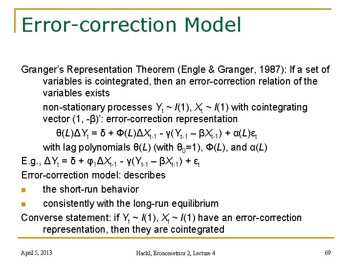
Error-correction Model Granger’s Representation Theorem (Engle & Granger, 1987): If a set of variables is cointegrated, then an error-correction (EC) relation of the variables exists non-stationary processes Yt ~ I(1), Xt ~ I(1) with cointegrating vector (1, -β)’: error-correction representation θ(L)ΔYt = δ + Φ(L)ΔXt-1 - γ(Yt-1 – βXt-1) + α(L)εt with white noise εt, lag polynomials θ(L) (with θ 0=1), Φ(L), and α(L) n Error-correction model: describes q q n n the short-run behaviour consistently with the long-run equilibrium Long-run equilibrium: Yt = βXt, deviations from equilibrium: Yt – βXt Converse statement: if Yt ~ I(1), Xt ~ I(1) have an error-correction representation, then they are cointegrated April 5, 2013 Hackl, Econometrics 2, Lecture 4 49

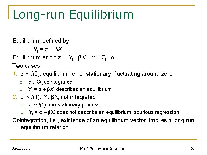
Long-run Equilibrium defined by Yt = α + βXt Equilibrium error: zt = Yt - βXt - α = Zt - α Two cases: 1. zt ~ I(0): equilibrium error stationary, fluctuating around zero q q Yt, βXt cointegrated Yt = α + βXt describes an equilibrium 2. zt ~ I(1), Yt, βXt not integrated q q zt ~ I(1) non-stationary process Yt = α + βXt does not describe an equilibrium, spurious regression Cointegration, i. e. , existence of an equilibrium vector, implies a long-run equilibrium relation April 5, 2013 Hackl, Econometrics 2, Lecture 4 50

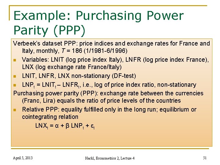
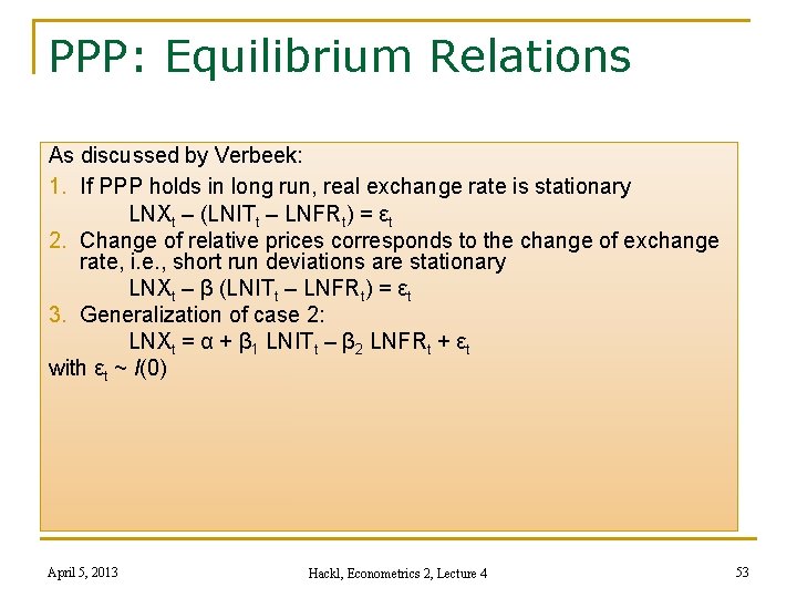
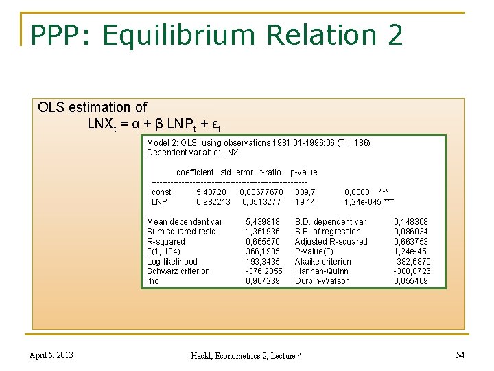
Example: Purchasing Power Parity (PPP) Verbeek’s dataset PPP: price indices and exchange rates for France and Italy, monthly, T = 186 (1/1981 -6/1996) n Variables: LNIT (log price index Italy), LNFR (log price index France), LNX (log exchange rate France/Italy) n LNIT, LNFR, LNX non-stationary (DF-test) n LNPt = LNITt – LNFRt, i. e. , log of price index ratio, non-stationary Purchasing power parity (PPP): exchange rate between the currencies (Franc, Lira) equals the ratio of price levels of the countries n Relative PPP: equality fulfilled only in the long run; equilibrium or cointegrating relation LNXt = α + β LNPt + εt April 5, 2013 Hackl, Econometrics 2, Lecture 4 51

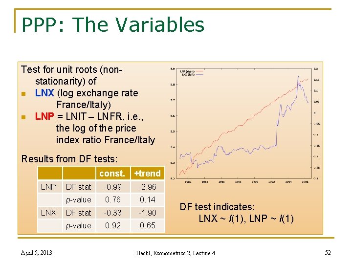
PPP: The Variables Test for unit roots (nonstationarity) of n LNX (log exchange rate France/Italy) n LNP = LNIT – LNFR, i. e. , the log of the price index ratio France/Italy Results from DF tests: const. +trend LNP LNX April 5, 2013 DF stat -0. 99 -2. 96 p-value 0. 76 0. 14 DF stat -0. 33 -1. 90 p-value 0. 92 0. 65 DF test indicates: LNX ~ I(1), LNP ~ I(1) Hackl, Econometrics 2, Lecture 4 52

PPP: Equilibrium Relations As discussed by Verbeek: 1. If PPP holds in long run, real exchange rate is stationary LNXt – (LNITt – LNFRt) = εt 2. Change of relative prices corresponds to the change of exchange rate, i. e. , short run deviations are stationary LNXt – β (LNITt – LNFRt) = εt 3. Generalization of case 2: LNXt = α + β 1 LNITt – β 2 LNFRt + εt with εt ~ I(0) April 5, 2013 Hackl, Econometrics 2, Lecture 4 53

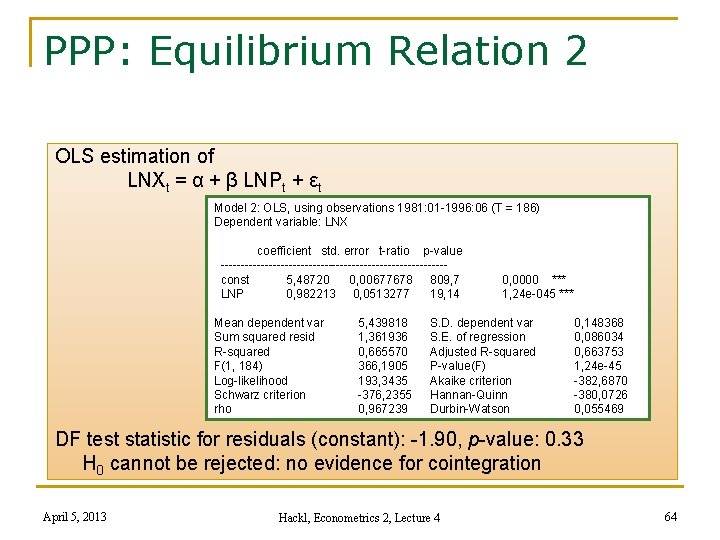
PPP: Equilibrium Relation 2 OLS estimation of LNXt = α + β LNPt + εt Model 2: OLS, using observations 1981: 01 -1996: 06 (T = 186) Dependent variable: LNX coefficient std. error t-ratio p-value ---------------------------- const 5, 48720 0, 00677678 809, 7 LNP 0, 982213 0, 0513277 19, 14 Mean dependent var Sum squared resid R-squared F(1, 184) Log-likelihood Schwarz criterion rho 5, 439818 1, 361936 0, 665570 366, 1905 193, 3435 -376, 2355 0, 967239 0, 0000 *** 1, 24 e-045 *** S. D. dependent var S. E. of regression Adjusted R-squared P-value(F) Akaike criterion Hannan-Quinn Durbin-Watson 0, 148368 0, 086034 0, 663753 1, 24 e-45 -382, 6870 -380, 0726 0, 055469 April 5, 2013 Hackl, Econometrics 2, Lecture 4 54

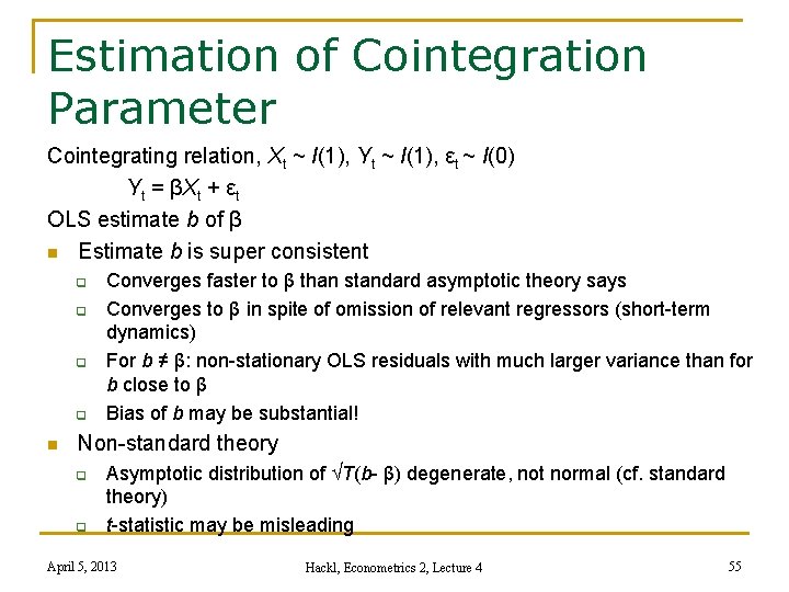
Estimation of Cointegration Parameter Cointegrating relation, Xt ~ I(1), Yt ~ I(1), εt ~ I(0) Yt = βXt + εt OLS estimate b of β n Estimate b is super consistent q q n Converges faster to β than standard asymptotic theory says Converges to β in spite of omission of relevant regressors (short-term dynamics) For b ≠ β: non-stationary OLS residuals with much larger variance than for b close to β Bias of b may be substantial! Non-standard theory q q Asymptotic distribution of √T(b- β) degenerate, not normal (cf. standard theory) t-statistic may be misleading April 5, 2013 Hackl, Econometrics 2, Lecture 4 55

Estimation of Spurious Regression Parameter Non-stationary processes Xt ~ I(1), Yt ~ I(1) Yt = βXt + εt Spurious regression, εt ~ I(1) OLS estimate b of β n Non-standard distribution n Large values of R 2, t-statistic n Highly autocorrelated residuals n DW statistic close to zero Remedy: add lagged regressors, e. g. , Yt-1 n n For Yt = δ + θYt-1 + φ0 Xt + φ1 Xt-1 + εt, parameter values can be found such that εt ~ I(0) Consistent estimates April 5, 2013 Hackl, Econometrics 2, Lecture 4 56

Contents n n n n n Dynamic Models Lag Structure: Estimation ADL Models for Expectations Models with Non-stationary Variables Cointegration Test for Cointegration Error-correction Model April 5, 2013 Hackl, Econometrics 2, Lecture 4 57

Identification of Cointegration Information about cointegration n Economic theory n Visual inspection of data n Statistical tests April 5, 2013 Hackl, Econometrics 2, Lecture 4 58

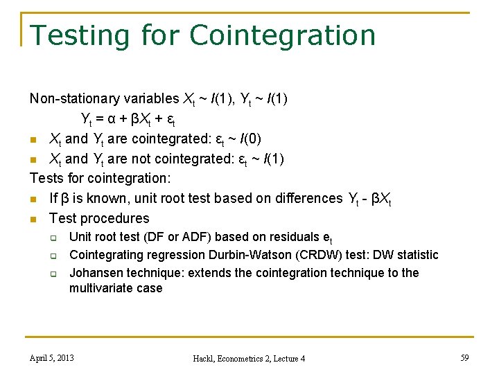
Testing for Cointegration Non-stationary variables Xt ~ I(1), Yt ~ I(1) Yt = α + βXt + εt n Xt and Yt are cointegrated: εt ~ I(0) n Xt and Yt are not cointegrated: εt ~ I(1) Tests for cointegration: n If β is known, unit root test based on differences Yt - βXt n Test procedures q q q Unit root test (DF or ADF) based on residuals et Cointegrating regression Durbin-Watson (CRDW) test: DW statistic Johansen technique: extends the cointegration technique to the multivariate case April 5, 2013 Hackl, Econometrics 2, Lecture 4 59

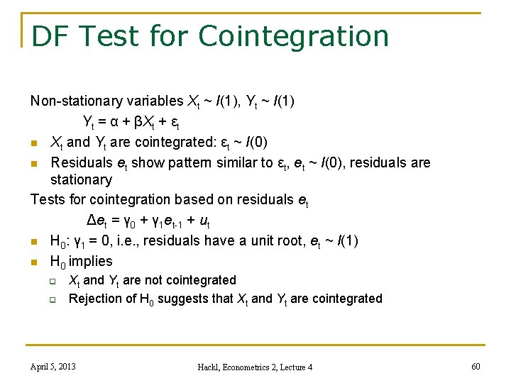
DF Test for Cointegration Non-stationary variables Xt ~ I(1), Yt ~ I(1) Yt = α + βXt + εt n Xt and Yt are cointegrated: εt ~ I(0) n Residuals et show pattern similar to εt, et ~ I(0), residuals are stationary Tests for cointegration based on residuals et Δet = γ 0 + γ 1 et-1 + ut n H 0: γ 1 = 0, i. e. , residuals have a unit root, et ~ I(1) n H 0 implies q q Xt and Yt are not cointegrated Rejection of H 0 suggests that Xt and Yt are cointegrated April 5, 2013 Hackl, Econometrics 2, Lecture 4 60

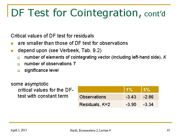
DF Test for Cointegration, cont’d Critical values of DF test for residuals n are smaller than those of DF test for observations n depend upon (see Verbeek, Tab. 9. 2) q q q number of elements of cointegrating vector (including left-hand side), K number of observations T significance level some asymptotic critical values for the DFtest with constant term April 5, 2013 1% 5% Observations -3. 43 -2. 86 Residuals, K=2 -3. 90 -3. 34 Hackl, Econometrics 2, Lecture 4 61

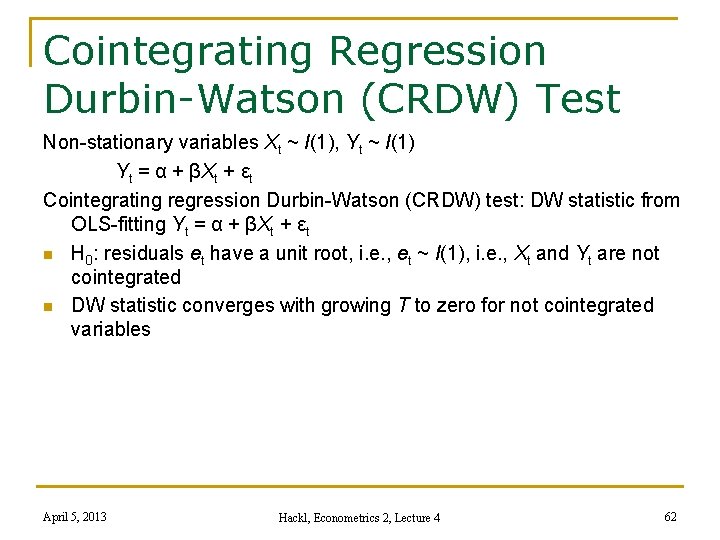
Cointegrating Regression Durbin-Watson (CRDW) Test Non-stationary variables Xt ~ I(1), Yt ~ I(1) Yt = α + βXt + εt Cointegrating regression Durbin-Watson (CRDW) test: DW statistic from OLS-fitting Yt = α + βXt + εt n H 0: residuals et have a unit root, i. e. , et ~ I(1), i. e. , Xt and Yt are not cointegrated n DW statistic converges with growing T to zero for not cointegrated variables April 5, 2013 Hackl, Econometrics 2, Lecture 4 62

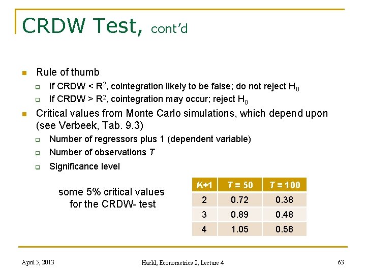
CRDW Test, n Rule of thumb q q n cont’d If CRDW < R 2, cointegration likely to be false; do not reject H 0 If CRDW > R 2, cointegration may occur; reject H 0 Critical values from Monte Carlo simulations, which depend upon (see Verbeek, Tab. 9. 3) q Number of regressors plus 1 (dependent variable) Number of observations T q Significance level q some 5% critical values for the CRDW- test April 5, 2013 K+1 T = 50 T = 100 2 0. 72 0. 38 3 0. 89 0. 48 4 1. 05 0. 58 Hackl, Econometrics 2, Lecture 4 63

PPP: Equilibrium Relation 2 OLS estimation of LNXt = α + β LNPt + εt Model 2: OLS, using observations 1981: 01 -1996: 06 (T = 186) Dependent variable: LNX coefficient std. error t-ratio p-value ---------------------------- const 5, 48720 0, 00677678 809, 7 LNP 0, 982213 0, 0513277 19, 14 Mean dependent var Sum squared resid R-squared F(1, 184) Log-likelihood Schwarz criterion rho 5, 439818 1, 361936 0, 665570 366, 1905 193, 3435 -376, 2355 0, 967239 0, 0000 *** 1, 24 e-045 *** S. D. dependent var S. E. of regression Adjusted R-squared P-value(F) Akaike criterion Hannan-Quinn Durbin-Watson 0, 148368 0, 086034 0, 663753 1, 24 e-45 -382, 6870 -380, 0726 0, 055469 DF test statistic for residuals (constant): -1. 90, p-value: 0. 33 H 0 cannot be rejected: no evidence for cointegration April 5, 2013 Hackl, Econometrics 2, Lecture 4 64

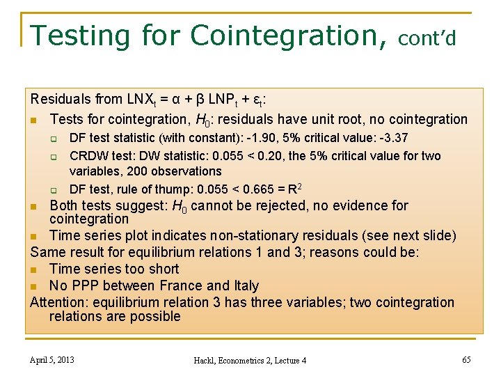
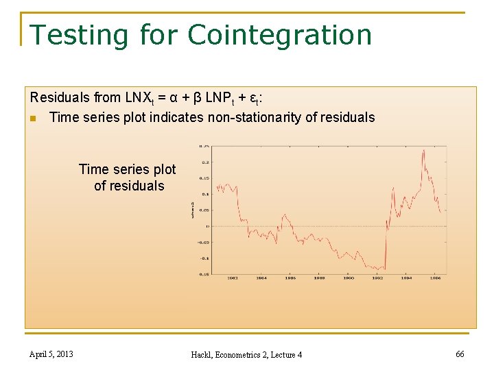
Testing for Cointegration, cont’d Residuals from LNXt = α + β LNPt + εt: n Tests for cointegration, H 0: residuals have unit root, no cointegration q q q DF test statistic (with constant): -1. 90, 5% critical value: -3. 37 CRDW test: DW statistic: 0. 055 < 0. 20, the 5% critical value for two variables, 200 observations DF test, rule of thump: 0. 055 < 0. 665 = R 2 Both tests suggest: H 0 cannot be rejected, no evidence for cointegration n Time series plot indicates non-stationary residuals (see next slide) Same result for equilibrium relations 1 and 3; reasons could be: n Time series too short n No PPP between France and Italy Attention: equilibrium relation 3 has three variables; two cointegration relations are possible n April 5, 2013 Hackl, Econometrics 2, Lecture 4 65

Testing for Cointegration Residuals from LNXt = α + β LNPt + εt: n Time series plot indicates non-stationarity of residuals Time series plot of residuals April 5, 2013 Hackl, Econometrics 2, Lecture 4 66

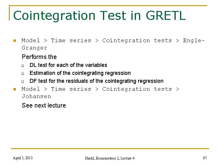
Cointegration Test in GRETL n Model > Time series > Cointegration tests > Engle. Granger Performs the q q q n DL test for each of the variables Estimation of the cointegrating regression DF test for the residuals of the cointegrating regression Model > Time series > Cointegration tests > Johansen See next lecture April 5, 2013 Hackl, Econometrics 2, Lecture 4 67

Contents n n n n n Dynamic Models Lag Structure: Estimation ADL Models for Expectations Models with Non-stationary Variables Cointegration Test for Cointegration Error-correction Model April 5, 2013 Hackl, Econometrics 2, Lecture 4 68

Error-correction Model Granger’s Representation Theorem (Engle & Granger, 1987): If a set of variables is cointegrated, then an error-correction relation of the variables exists non-stationary processes Yt ~ I(1), Xt ~ I(1) with cointegrating vector (1, -β)’: error-correction representation θ(L)ΔYt = δ + Φ(L)ΔXt-1 - γ(Yt-1 – βXt-1) + α(L)εt with lag polynomials θ(L) (with θ 0=1), Φ(L), and α(L) E. g. , ΔYt = δ + φ1ΔXt-1 - γ(Yt-1 – βXt-1) + εt Error-correction model: describes n the short-run behavior n consistently with the long-run equilibrium Converse statement: if Yt ~ I(1), Xt ~ I(1) have an error-correction representation, then they are cointegrated April 5, 2013 Hackl, Econometrics 2, Lecture 4 69

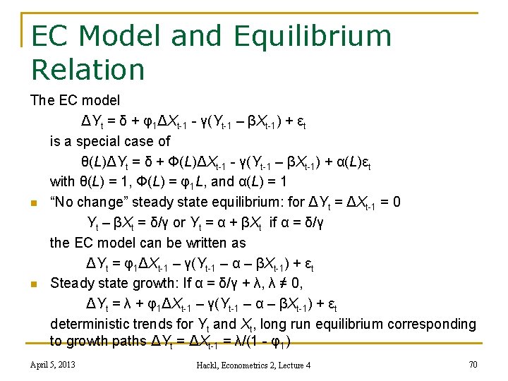
EC Model and Equilibrium Relation The EC model ΔYt = δ + φ1ΔXt-1 - γ(Yt-1 – βXt-1) + εt is a special case of θ(L)ΔYt = δ + Φ(L)ΔXt-1 - γ(Yt-1 – βXt-1) + α(L)εt with θ(L) = 1, Φ(L) = φ1 L, and α(L) = 1 n “No change” steady state equilibrium: for ΔYt = ΔXt-1 = 0 Yt – βXt = δ/γ or Yt = α + βXt if α = δ/γ the EC model can be written as ΔYt = φ1ΔXt-1 – γ(Yt-1 – α – βXt-1) + εt n Steady state growth: If α = δ/γ + λ, λ ≠ 0, ΔYt = λ + φ1ΔXt-1 – γ(Yt-1 – α – βXt-1) + εt deterministic trends for Yt and Xt, long run equilibrium corresponding to growth paths ΔYt = ΔXt-1 = λ/(1 - φ1) April 5, 2013 Hackl, Econometrics 2, Lecture 4 70

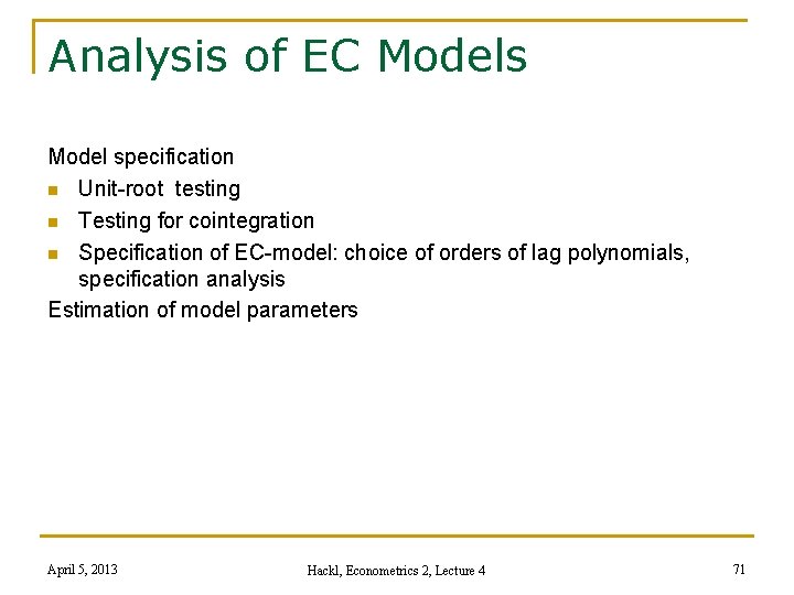
Analysis of EC Models Model specification n Unit-root testing n Testing for cointegration n Specification of EC-model: choice of orders of lag polynomials, specification analysis Estimation of model parameters April 5, 2013 Hackl, Econometrics 2, Lecture 4 71

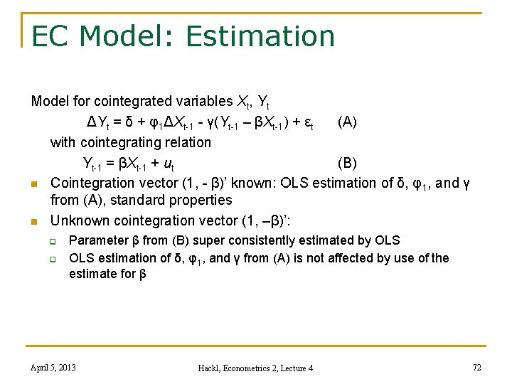
EC Model: Estimation Model for cointegrated variables Xt, Yt ΔYt = δ + φ1ΔXt-1 - γ(Yt-1 – βXt-1) + εt (A) with cointegrating relation Yt-1 = βXt-1 + ut (B) n Cointegration vector (1, - β)’ known: OLS estimation of δ, φ 1, and γ from (A), standard properties n Unknown cointegration vector (1, –β)’: q q Parameter β from (B) super consistently estimated by OLS estimation of δ, φ1, and γ from (A) is not affected by use of the estimate for β April 5, 2013 Hackl, Econometrics 2, Lecture 4 72

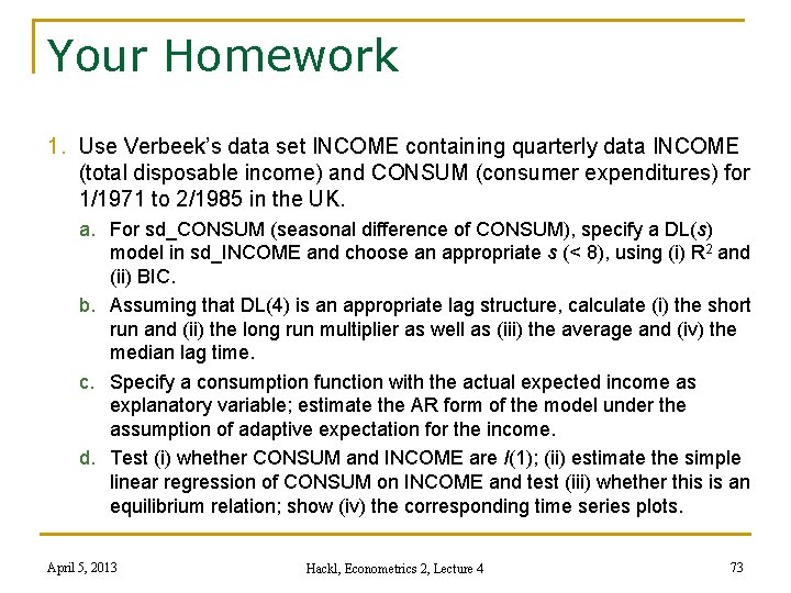
Your Homework 1. Use Verbeek’s data set INCOME containing quarterly data INCOME (total disposable income) and CONSUM (consumer expenditures) for 1/1971 to 2/1985 in the UK. a. For sd_CONSUM (seasonal difference of CONSUM), specify a DL(s) model in sd_INCOME and choose an appropriate s (< 8), using (i) R 2 and (ii) BIC. b. Assuming that DL(4) is an appropriate lag structure, calculate (i) the short run and (ii) the long run multiplier as well as (iii) the average and (iv) the median lag time. c. Specify a consumption function with the actual expected income as explanatory variable; estimate the AR form of the model under the assumption of adaptive expectation for the income. d. Test (i) whether CONSUM and INCOME are I(1); (ii) estimate the simple linear regression of CONSUM on INCOME and test (iii) whether this is an equilibrium relation; show (iv) the corresponding time series plots. April 5, 2013 Hackl, Econometrics 2, Lecture 4 73

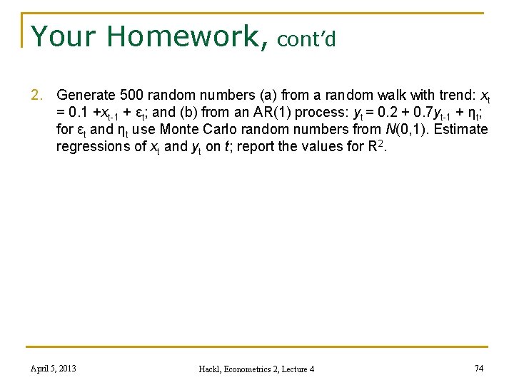
Your Homework, cont’d 2. Generate 500 random numbers (a) from a random walk with trend: xt = 0. 1 +xt-1 + εt; and (b) from an AR(1) process: yt = 0. 2 + 0. 7 yt-1 + ηt; for εt and ηt use Monte Carlo random numbers from N(0, 1). Estimate regressions of xt and yt on t; report the values for R 2. April 5, 2013 Hackl, Econometrics 2, Lecture 4 74