Dynamic Trees Goal maintain a forest of rooted

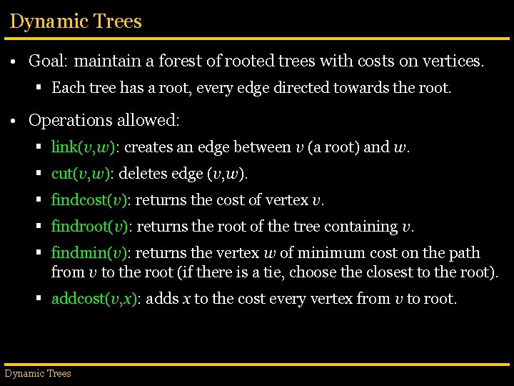
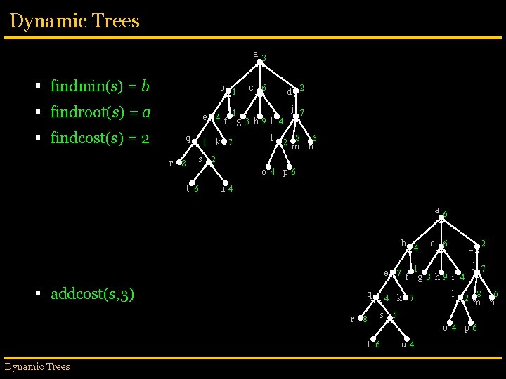
Dynamic Trees • Goal: maintain a forest of rooted trees with costs on vertices. § Each tree has a root, every edge directed towards the root. • Operations allowed: § link(v, w): creates an edge between v (a root) and w. § cut(v, w): deletes edge (v, w). § findcost(v): returns the cost of vertex v. § findroot(v): returns the root of the tree containing v. § findmin(v): returns the vertex w of minimum cost on the path from v to the root (if there is a tie, choose the closest to the root). § addcost(v, x): adds x to the cost every vertex from v to root. Dynamic Trees

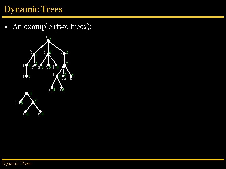
Dynamic Trees • An example (two trees): a 3 b 1 e 4 c f r l s 8 t 6 Dynamic Trees j 7 g 3 h 9 i 4 o 4 1 2 u 4 2 d 1 k 7 q 6 2 8 m p 6 6 n

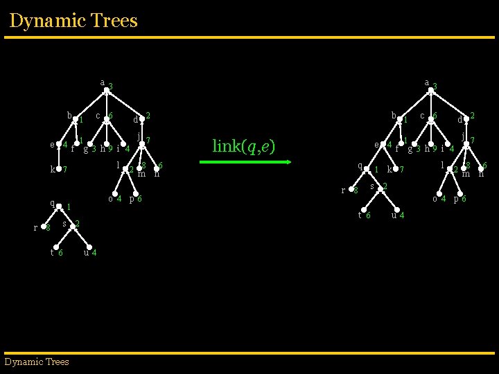
Dynamic Trees a 3 b 1 e 4 c r f l o 4 s t 6 Dynamic Trees b 1 2 d j 7 g 3 h 9 i 4 1 8 6 1 k 7 q a 3 2 8 m p 6 link(q, e) q 6 n r s 8 u 4 6 4 j 7 1 k 7 1 e f g 3 h 9 i 4 l 2 8 m 2 u 4 2 d o 4 t 6 2 c p 6 6 n

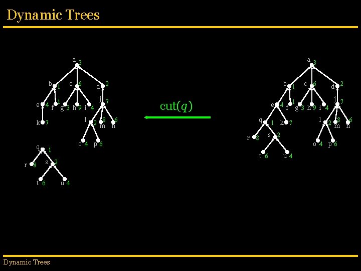
Dynamic Trees a 3 b 1 e 4 c r f l o 4 s t 6 Dynamic Trees b 1 2 d j 7 g 3 h 9 i 4 1 8 6 1 k 7 q a 3 2 8 m p 6 cut(q) q 6 n r s 8 u 4 6 4 j 7 1 k 7 1 e f g 3 h 9 i 4 l 2 8 m 2 u 4 2 d o 4 t 6 2 c p 6 6 n

Dynamic Trees a 3 § findmin(s) = b b 1 § findroot(s) = a § findcost(s) = 2 q r s 8 c 6 4 1 k 7 f g 3 h 9 i 4 l 2 8 m 6 n 2 o 4 t 6 j 7 1 e 2 d p 6 u 4 a 6 b 4 § addcost(s, 3) q r s 8 6 7 j 7 4 k 7 1 e f g 3 h 9 i 4 l 2 8 m 5 u 4 2 d o 4 t 6 Dynamic Trees c p 6 6 n

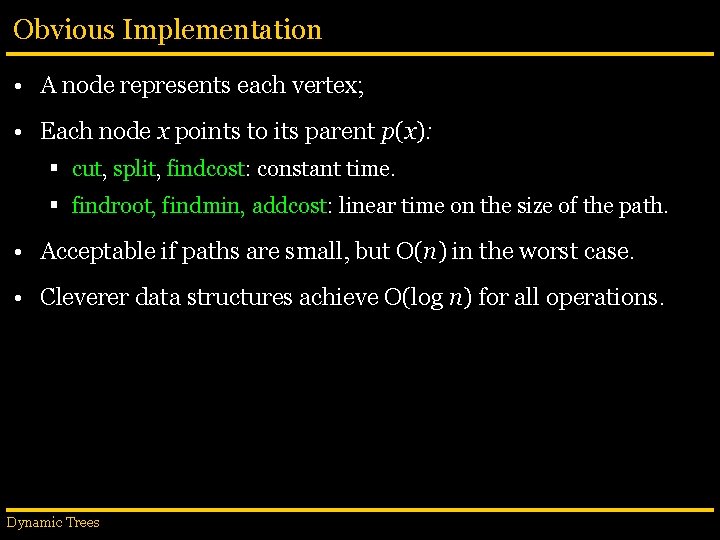
Obvious Implementation • A node represents each vertex; • Each node x points to its parent p(x): § cut, split, findcost: constant time. § findroot, findmin, addcost: linear time on the size of the path. • Acceptable if paths are small, but O(n) in the worst case. • Cleverer data structures achieve O(log n) for all operations. Dynamic Trees

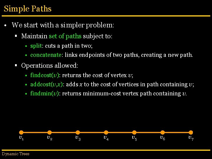
Simple Paths • We start with a simpler problem: § Maintain set of paths subject to: • split: cuts a path in two; • concatenate: links endpoints of two paths, creating a new path. § Operations allowed: • findcost(v): returns the cost of vertex v; • addcost(v, x): adds x to the cost of vertices in path containing v; • findmin(v): returns minimum-cost vertex path containing v. v 1 Dynamic Trees v 2 v 3 v 4 v 5 v 6 v 7

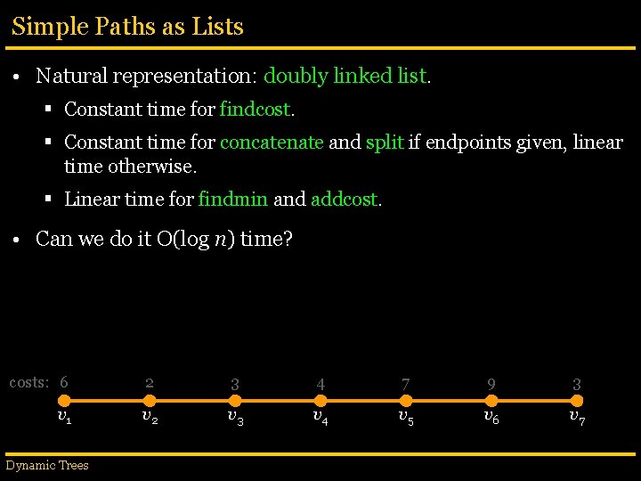
Simple Paths as Lists • Natural representation: doubly linked list. § Constant time for findcost. § Constant time for concatenate and split if endpoints given, linear time otherwise. § Linear time for findmin and addcost. • Can we do it O(log n) time? costs: 6 2 3 4 7 9 3 v 1 v 2 v 3 v 4 v 5 v 6 v 7 Dynamic Trees

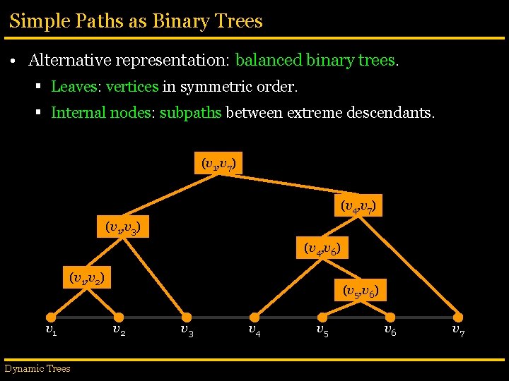
Simple Paths as Binary Trees • Alternative representation: balanced binary trees. § Leaves: vertices in symmetric order. § Internal nodes: subpaths between extreme descendants. (v 1, v 7) (v 4, v 7) (v 1, v 3) (v 4, v 6) (v 1, v 2) v 1 Dynamic Trees (v 5, v 6) v 2 v 3 v 4 v 5 v 6 v 7

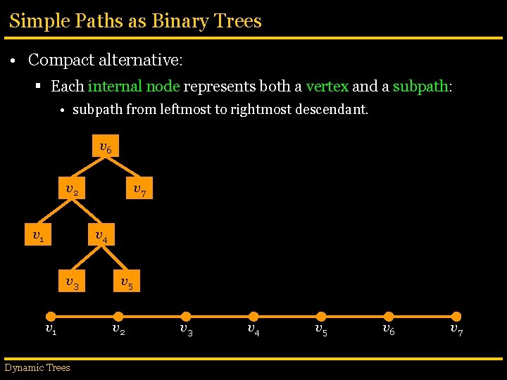
Simple Paths as Binary Trees • Compact alternative: § Each internal node represents both a vertex and a subpath: • subpath from leftmost to rightmost descendant. v 6 v 2 v 1 v 7 v 4 v 3 v 1 Dynamic Trees v 5 v 2 v 3 v 4 v 5 v 6 v 7

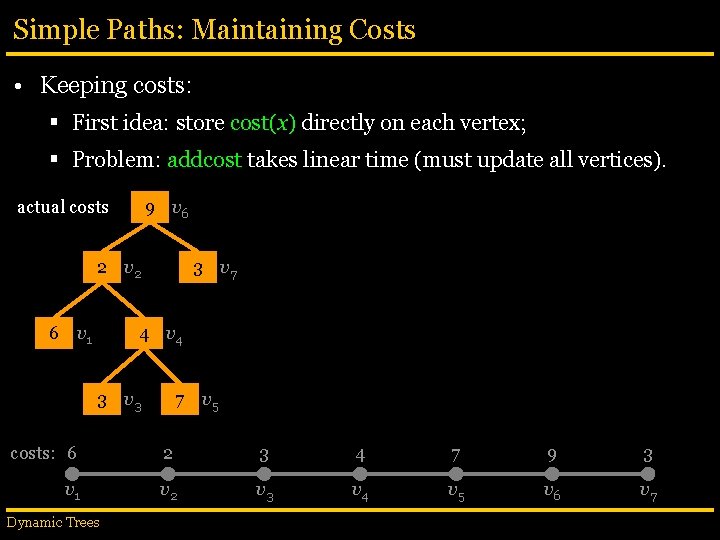
Simple Paths: Maintaining Costs • Keeping costs: § First idea: store cost(x) directly on each vertex; § Problem: addcost takes linear time (must update all vertices). actual costs 9 v 6 2 v 2 6 v 1 3 v 7 4 v 4 3 v 3 7 v 5 costs: 6 2 3 4 7 9 3 v 1 v 2 v 3 v 4 v 5 v 6 v 7 Dynamic Trees

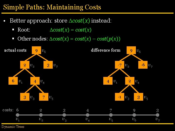
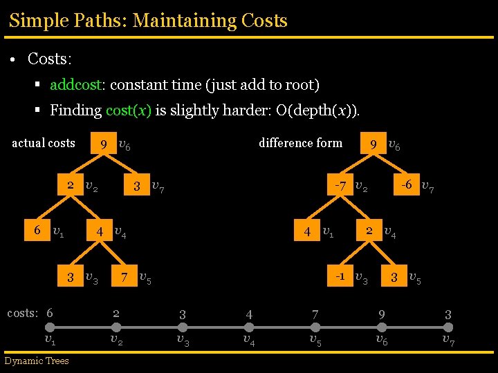
Simple Paths: Maintaining Costs • Better approach: store cost(x) instead: cost(x) = cost(x) § Root: § Other nodes: cost(x) = cost(x) – cost(p(x)) actual costs 9 v 6 2 v 2 6 v 1 difference form 3 v 7 -7 v 2 4 v 4 3 v 3 9 v 6 4 v 1 7 v 5 -6 v 7 2 v 4 -1 v 3 3 v 5 costs: 6 2 3 4 7 9 3 v 1 v 2 v 3 v 4 v 5 v 6 v 7 Dynamic Trees

Simple Paths: Maintaining Costs • Costs: § addcost: constant time (just add to root) § Finding cost(x) is slightly harder: O(depth(x)). actual costs 9 v 6 2 v 2 6 v 1 difference form 3 v 7 -7 v 2 4 v 4 3 v 3 9 v 6 4 v 1 7 v 5 -6 v 7 2 v 4 -1 v 3 3 v 5 costs: 6 2 3 4 7 9 3 v 1 v 2 v 3 v 4 v 5 v 6 v 7 Dynamic Trees

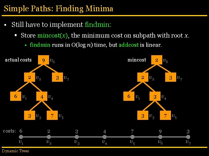
Simple Paths: Finding Minima • Still have to implement findmin: § Store mincost(x), the minimum cost on subpath with root x. • findmin runs in O(log n) time, but addcost is linear. actual costs 9 v 6 2 v 2 6 v 1 mincost 3 v 7 2 v 2 4 v 4 3 v 3 2 v 6 6 v 1 7 v 5 3 v 7 3 v 4 3 v 3 7 v 5 costs: 6 2 3 4 7 9 3 v 1 v 2 v 3 v 4 v 5 v 6 v 7 Dynamic Trees

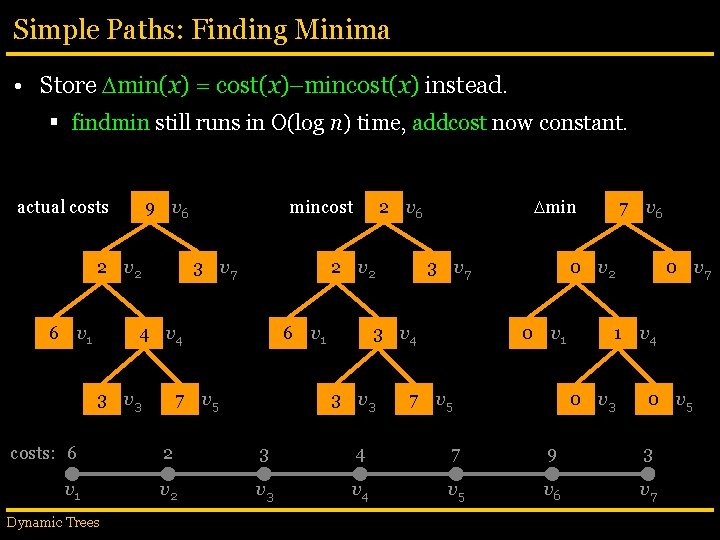
Simple Paths: Finding Minima • Store min(x) = cost(x)–mincost(x) instead. § findmin still runs in O(log n) time, addcost now constant. actual costs 9 v 6 2 v 2 6 v 1 mincost 3 v 7 2 v 2 4 v 4 3 v 3 6 v 1 7 v 5 min 2 v 6 3 v 7 3 v 4 3 v 3 7 v 6 0 v 2 0 v 1 7 v 5 0 v 7 1 v 4 0 v 3 0 v 5 costs: 6 2 3 4 7 9 3 v 1 v 2 v 3 v 4 v 5 v 6 v 7 Dynamic Trees

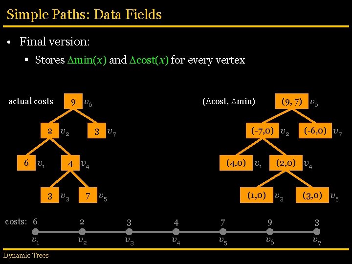
Simple Paths: Data Fields • Final version: § Stores min(x) and cost(x) for every vertex actual costs 2 v 2 6 v 1 ( cost, min) 9 v 6 3 v 7 (-7, 0) v 2 4 v 4 3 v 3 (9, 7) v 6 (4, 0) v 1 7 v 5 (-6, 0) v 7 (2, 0) v 4 (1, 0) v 3 (3, 0) v 5 costs: 6 2 3 4 7 9 3 v 1 v 2 v 3 v 4 v 5 v 6 v 7 Dynamic Trees

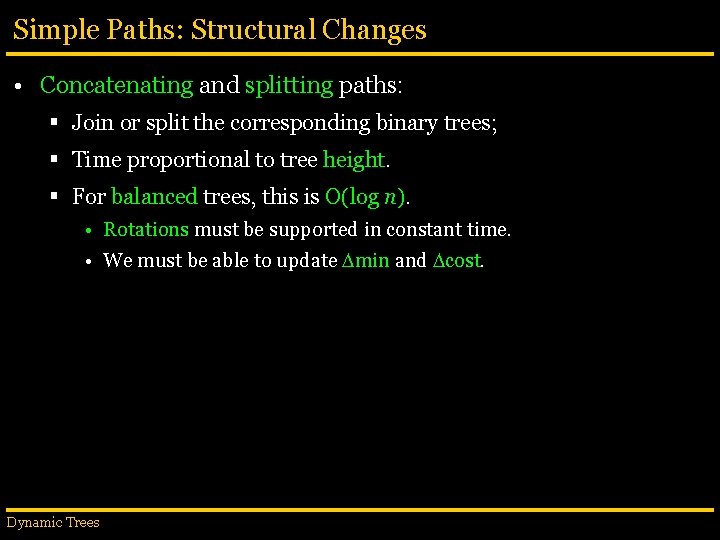
Simple Paths: Structural Changes • Concatenating and splitting paths: § Join or split the corresponding binary trees; § Time proportional to tree height. § For balanced trees, this is O(log n). • Rotations must be supported in constant time. • We must be able to update min and cost. Dynamic Trees

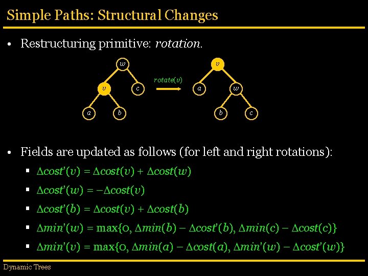
Simple Paths: Structural Changes • Restructuring primitive: rotation. w v rotate(v) v a c b a w b c • Fields are updated as follows (for left and right rotations): § cost’(v) = cost(v) + cost(w) § cost’(w) = – cost(v) § cost’(b) = cost(v) + cost(b) § min’(w) = max{0, min(b) – cost’(b), min(c) – cost(c)} § min’(v) = max{0, min(a) – cost(a), min’(w) – cost’(w)} Dynamic Trees

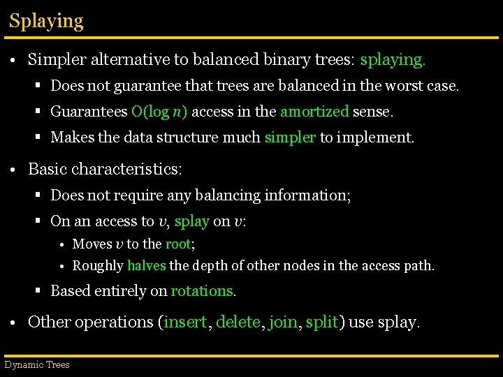
Splaying • Simpler alternative to balanced binary trees: splaying. § Does not guarantee that trees are balanced in the worst case. § Guarantees O(log n) access in the amortized sense. § Makes the data structure much simpler to implement. • Basic characteristics: § Does not require any balancing information; § On an access to v, splay on v: • Moves v to the root; • Roughly halves the depth of other nodes in the access path. § Based entirely on rotations. • Other operations (insert, delete, join, split) use splay. Dynamic Trees

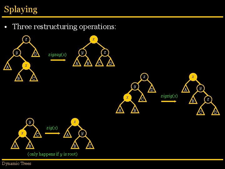
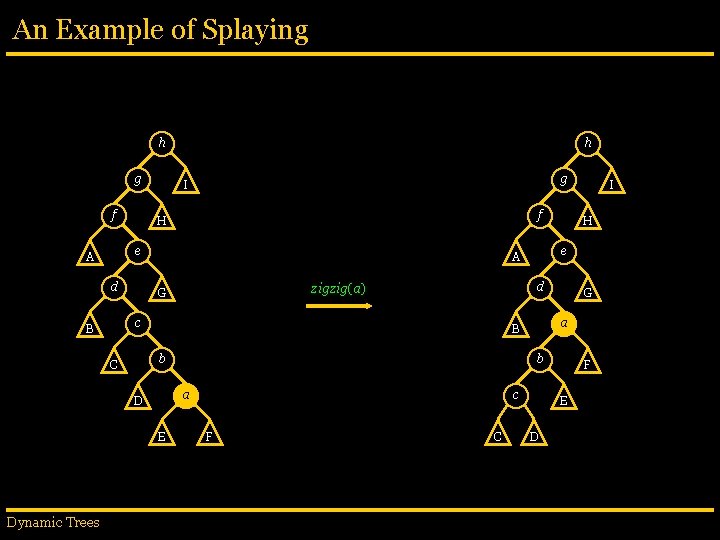
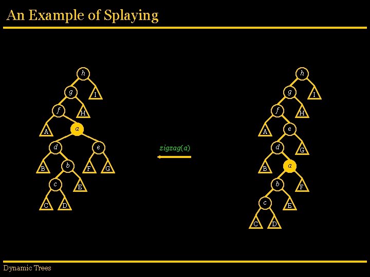
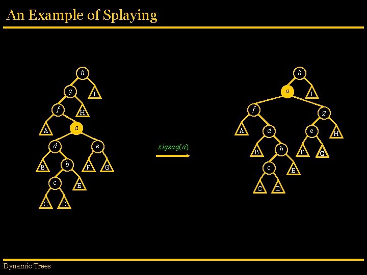
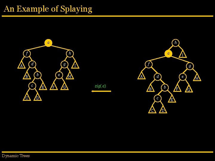
Splaying • Three restructuring operations: z x y D A x A y zigzag(x) B z B C D z C y x A y x zig(x) x A C B y A B (only happens if y is root) Dynamic Trees C D C B x y A zigzig(x) z B C D

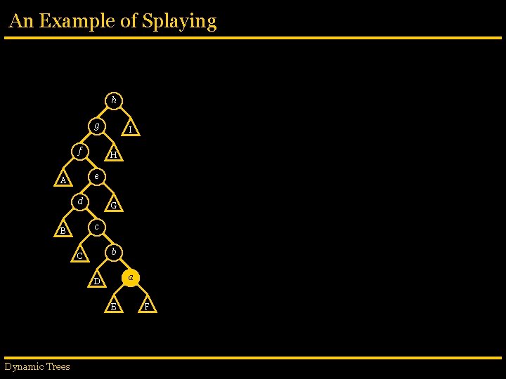
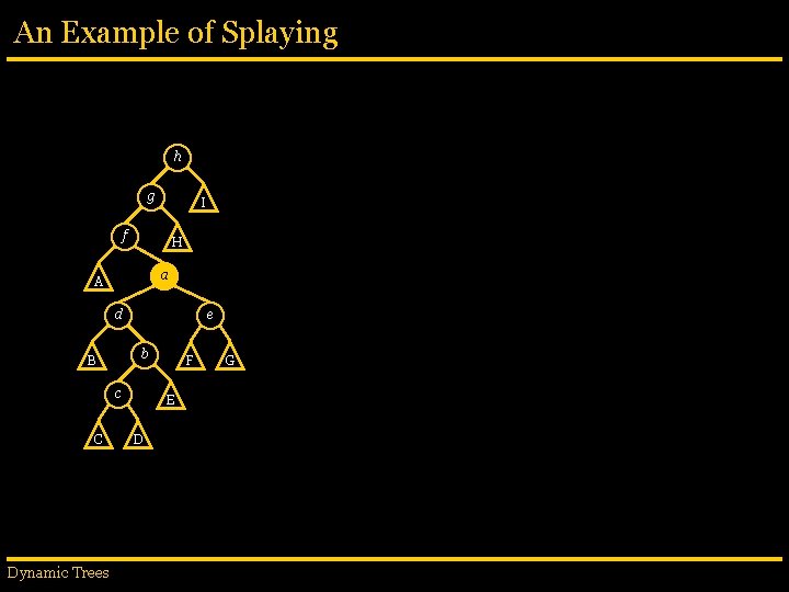
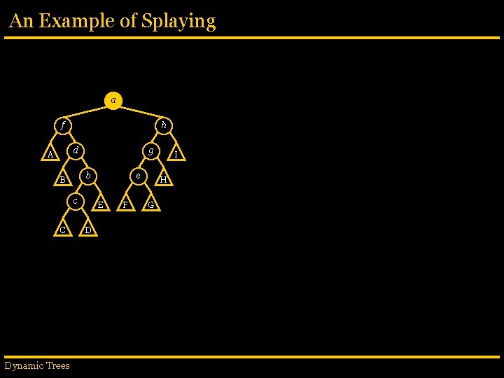
An Example of Splaying h g f I H e A d G c B b C a D E Dynamic Trees F

An Example of Splaying h g f g I f H e A d b a D E G a B b C H d zigzig(a) G c F C I e A c B Dynamic Trees h F E D

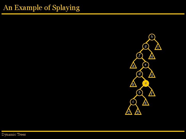
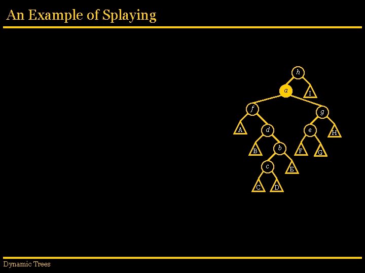
An Example of Splaying h g f H e A d G a B b c C Dynamic Trees I F E D

An Example of Splaying h h g f f H a A e b B c F G G a B b E c D C Dynamic Trees H d zigzag(a) I e A d C g I F E D

An Example of Splaying h g I f H a A d e b B c C Dynamic Trees F E D G

An Example of Splaying h h g f a e b c Dynamic Trees F E D g A d B I f H A C a I zigzag(a) d b B G e c C F E D H G

An Example of Splaying h a I f g A d e b B c C Dynamic Trees F E D H G

An Example of Splaying a h f h d A g b B c C e E F a f I H G g A zig(a) d D e b B c C Dynamic Trees I F E D H G

An Example of Splaying a f h d A g b B c C Dynamic Trees e E D F I H G

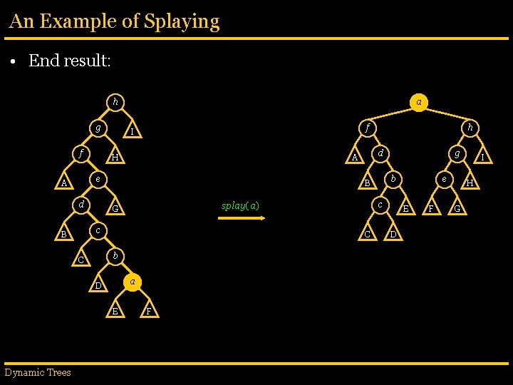
An Example of Splaying • End result: h g f f I H d C b C c splay(a) G a D E F g b B c B h d A e A Dynamic Trees a e E D F I H G

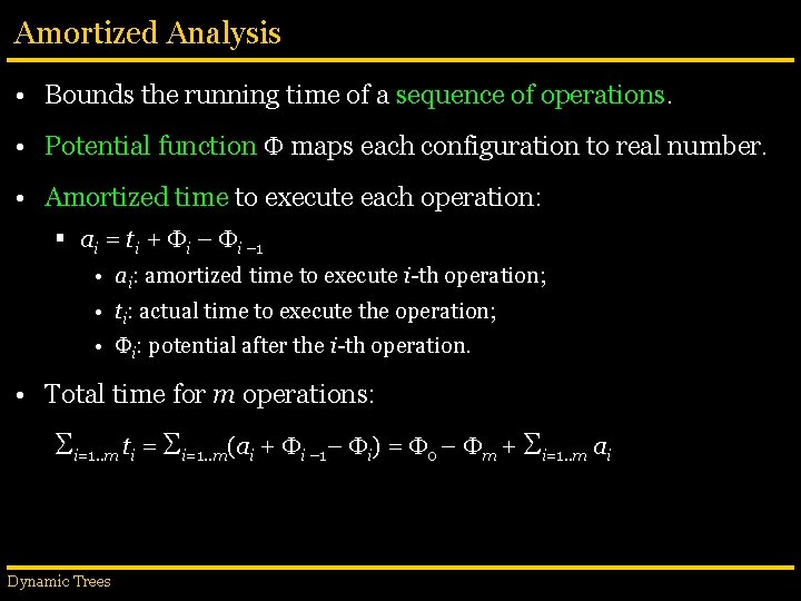
Amortized Analysis • Bounds the running time of a sequence of operations. • Potential function maps each configuration to real number. • Amortized time to execute each operation: § ai = ti + i – 1 • ai: amortized time to execute i-th operation; • ti: actual time to execute the operation; • i: potential after the i-th operation. • Total time for m operations: i=1. . m ti = i=1. . m(ai + i – 1– i) = 0 – m + i=1. . m ai Dynamic Trees

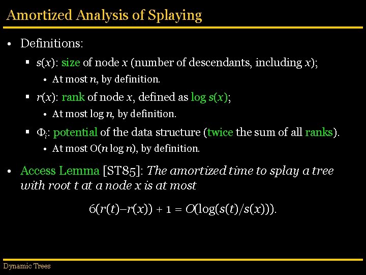
Amortized Analysis of Splaying • Definitions: § s(x): size of node x (number of descendants, including x); • At most n, by definition. § r(x): rank of node x, defined as log s(x); • At most log n, by definition. § i: potential of the data structure (twice the sum of all ranks). • At most O(n log n), by definition. • Access Lemma [ST 85]: The amortized time to splay a tree with root t at a node x is at most 6(r(t)–r(x)) + 1 = O(log(s(t)/s(x))). Dynamic Trees

Proof of Access Lemma • Access Lemma [ST 85]: The amortized time to splay a tree with root t at a node x is at most 6(r(t)–r(x)) + 1 = O(log(s(t)/s(x))). • Proof idea: § ri(x) = rank of x after the i-th splay step; § ai = amortized cost of the i-th splay step; § ai 6(ri(x)–ri– 1(x)) + 1 (for the zig step, if any) § ai 6(ri(x)–ri– 1(x)) (for any zig-zig and zig-zag steps) § Total amortized time for all k steps: i=1. . k ai i=1. . k-1 [6(ri(x)–ri– 1(x))] + [6(rk(x)–rk– 1(x)) + 1] = 6 rk(x) – 6 r 0(x) + 1 Dynamic Trees

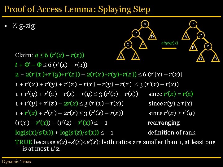
Proof of Access Lemma: Splaying Step • Zig-zig: z y x Claim: a 6 (r’(x) – r(x)) A x D C y A zigzig(x) z B B C t + ’ – 6 (r’(x) – r(x)) D 2 + 2(r’(x )+r’(y)+r’(z )) – 2(r(x )+r(y)+r(z )) 6 (r’(x) – r(x)) 1 + r’(x ) + r’(y) + r’(z ) – r(x ) – r(y) – r(z ) 3 (r’(x) – r(x)) 1 + r’(y) + r’(z ) – r(x) – r(y) 3 (r’(x) – r(x)) since r’(x) = r(z) 1 + r’(y) + r’(z ) – 2 r(x) 3 (r’(x) – r(x)) since r(y) r(x) 1 + r’(x) + r’(z ) – 2 r(x) 3 (r’(x) – r(x)) since r’(x) r’(y) (r(x ) – r’(x)) + (r’(z) – r’(x)) – 1 rearranging log(s(x)/s’(x)) + log(s’(z)/s’(x)) – 1 definition of rank TRUE because s(x)+s’(z)<s’(x): both ratios are smaller than 1, at least one is at most 1/2. Dynamic Trees

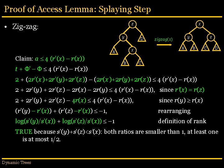
Proof of Access Lemma: Splaying Step z • Zig-zag: y t + ’ – 4 (r’(x) – r(x)) D B y zigzag(x) A x A Claim: a 4 (r’(x) – r(x)) x z B C D C 2 + (2 r’(x )+2 r’(y)+2 r’(z )) – (2 r(x )+2 r(y)+2 r(z )) 4 (r’(x) – r(x)) 2 + 2 r’(y) + 2 r’(z ) – 2 r(x) – 2 r(y) 4 (r’(x) – r(x)), since r’(x) = r(z) 2 + 2 r’(y) + 2 r’(z ) – 4 r(x) 4 (r’(x) – r(x)), since r(y) r(x) (r’(y) – r’(x)) + (r’(z) –r’(x)) – 1, rearranging log(s’(y)/s’(x)) + log(s’(z)/s’(x)) – 1 definition of rank TRUE because s’(y)+s’(z)<s’(x): both ratios are smaller than 1, at least one is at most 1/2. Dynamic Trees

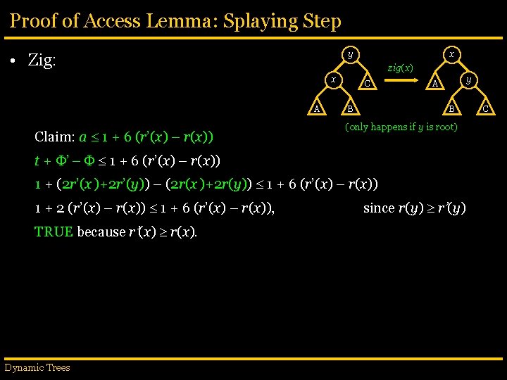
Proof of Access Lemma: Splaying Step y • Zig: zig(x) x A Claim: a 1 + 6 (r’(x) – r(x)) x C B y A B (only happens if y is root) t + ’ – 1 + 6 (r’(x) – r(x)) 1 + (2 r’(x )+2 r’(y)) – (2 r(x )+2 r(y)) 1 + 6 (r’(x) – r(x)) 1 + 2 (r’(x) – r(x)) 1 + 6 (r’(x) – r(x)), TRUE because r’(x) r(x). Dynamic Trees since r(y) r’(y) C

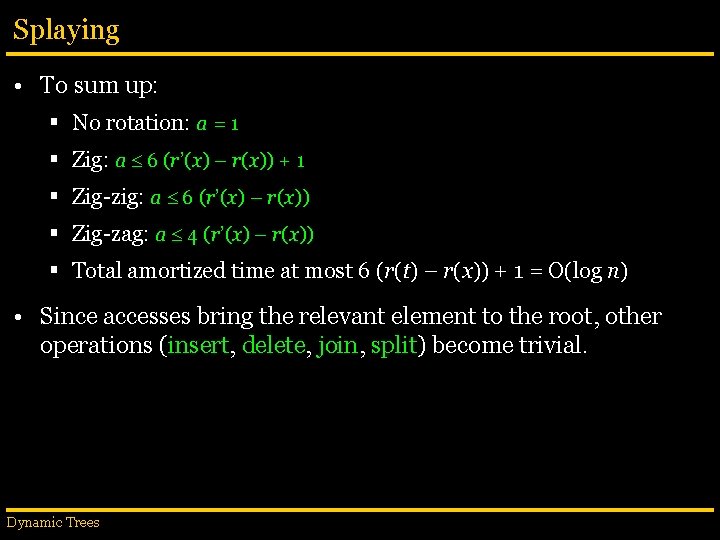
Splaying • To sum up: § No rotation: a = 1 § Zig: a 6 (r’(x) – r(x)) + 1 § Zig-zig: a 6 (r’(x) – r(x)) § Zig-zag: a 4 (r’(x) – r(x)) § Total amortized time at most 6 (r(t) – r(x)) + 1 = O(log n) • Since accesses bring the relevant element to the root, other operations (insert, delete, join, split) become trivial. Dynamic Trees

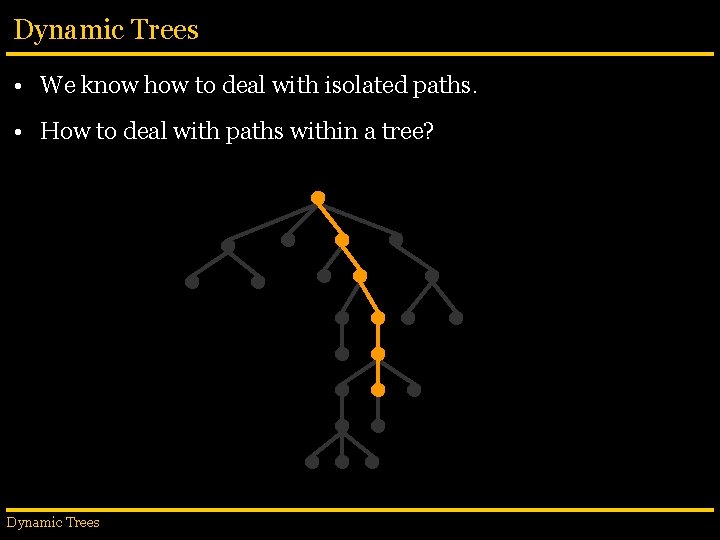
Dynamic Trees • We know how to deal with isolated paths. • How to deal with paths within a tree? Dynamic Trees

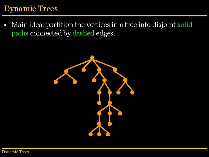
Dynamic Trees • Main idea: partition the vertices in a tree into disjoint solid paths connected by dashed edges. Dynamic Trees

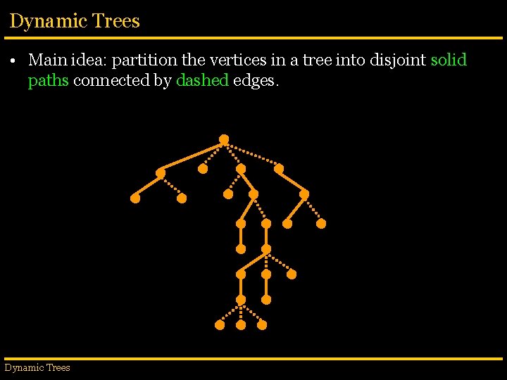
Dynamic Trees • Main idea: partition the vertices in a tree into disjoint solid paths connected by dashed edges. Dynamic Trees

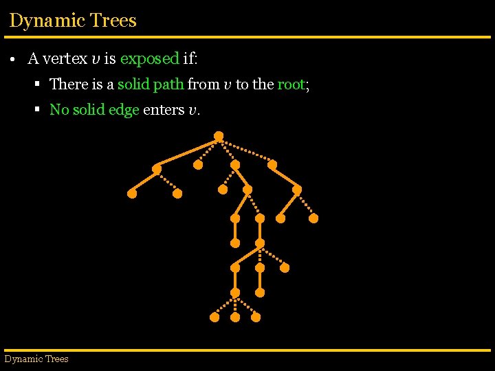
Dynamic Trees • A vertex v is exposed if: § There is a solid path from v to the root; § No solid edge enters v. Dynamic Trees

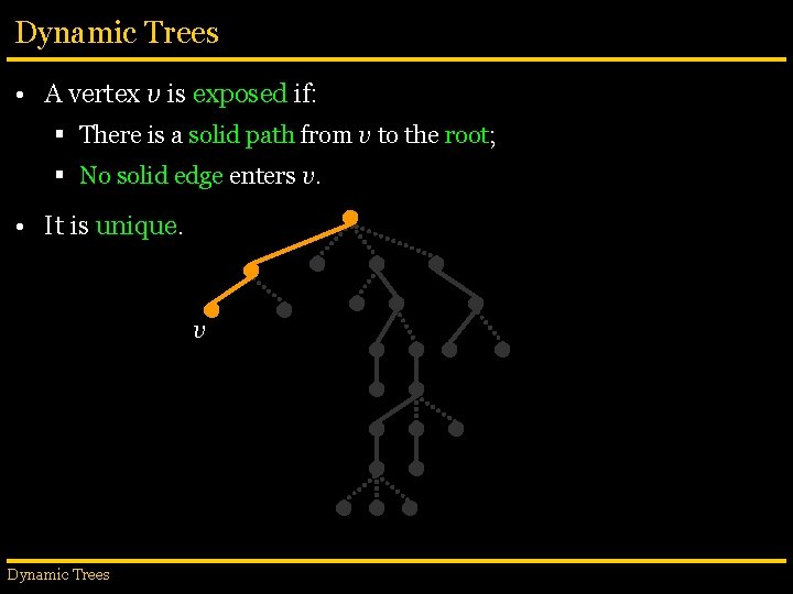
Dynamic Trees • A vertex v is exposed if: § There is a solid path from v to the root; § No solid edge enters v. • It is unique. v Dynamic Trees

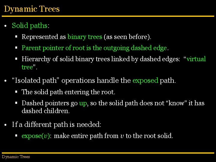
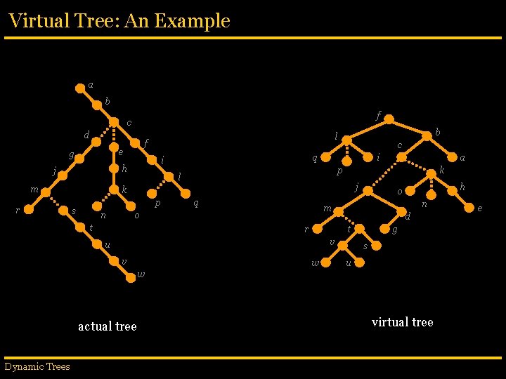
Dynamic Trees • Solid paths: § Represented as binary trees (as seen before). § Parent pointer of root is the outgoing dashed edge. § Hierarchy of solid binary trees linked by dashed edges: “virtual tree”. • “Isolated path” operations handle the exposed path. § The solid path entering the root. § Dashed pointers go up, so the solid path does not “know” it has dashed children. • If a different path is needed: § expose(v): make entire path from v to the root solid. Dynamic Trees

Virtual Tree: An Example a b f c d m c q i h j r f e g b l i p l k j k p s n q r n d t v u v w h o m o t a g s u w actual tree Dynamic Trees virtual tree e

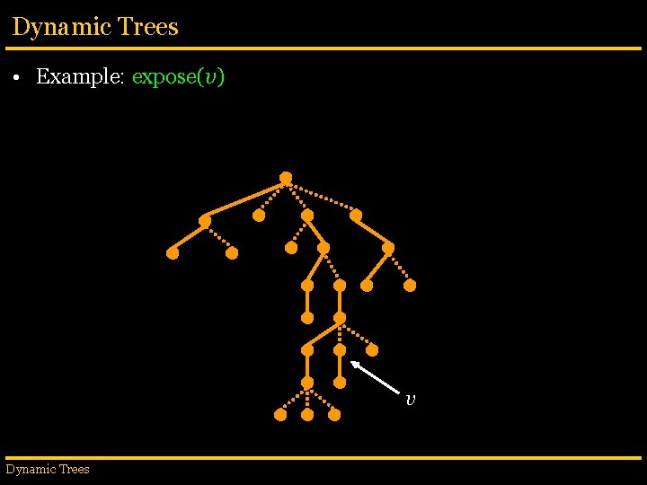
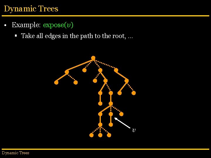
Dynamic Trees • Example: expose(v) v Dynamic Trees

Dynamic Trees • Example: expose(v) § Take all edges in the path to the root, … v Dynamic Trees

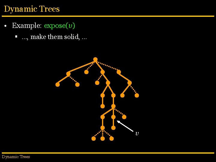
Dynamic Trees • Example: expose(v) § …, make them solid, … v Dynamic Trees

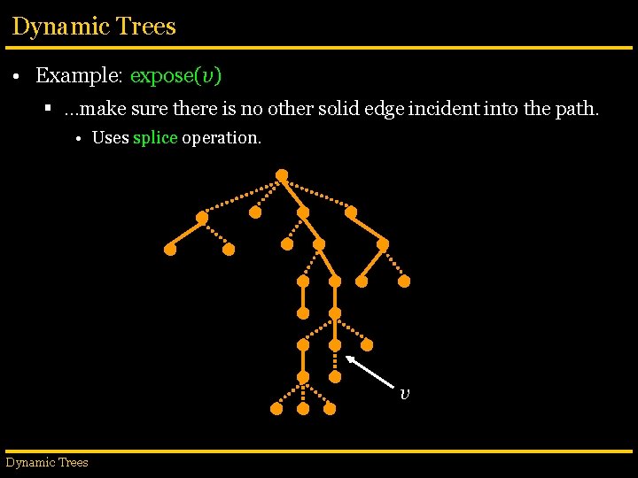
Dynamic Trees • Example: expose(v) § …make sure there is no other solid edge incident into the path. • Uses splice operation. v Dynamic Trees

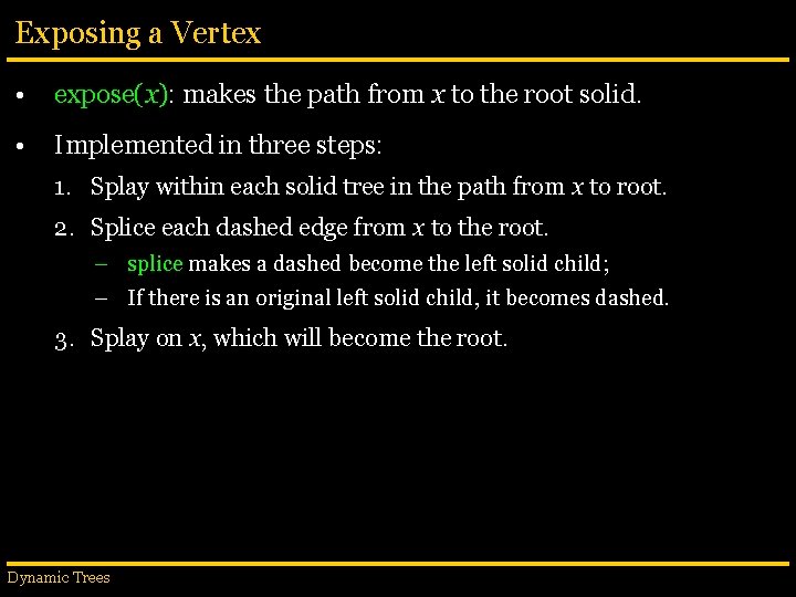
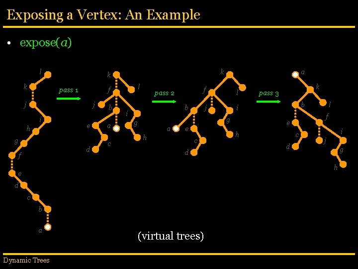
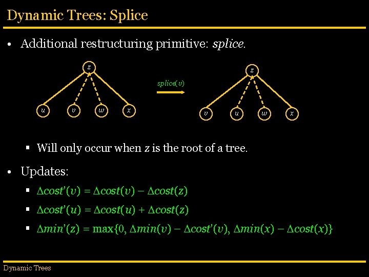
Exposing a Vertex • expose(x): makes the path from x to the root solid. • Implemented in three steps: 1. Splay within each solid tree in the path from x to root. 2. Splice each dashed edge from x to the root. – splice makes a dashed become the left solid child; – If there is an original left solid child, it becomes dashed. 3. Splay on x, which will become the root. Dynamic Trees

Exposing a Vertex: An Example • expose(a) l k pass 1 j h e g d f l f j i k k b a c pass 2 f l j i b i a g g a e h c d k pass 3 b f e h c d l i j g h e d c b a Dynamic Trees (virtual trees)

Dynamic Trees: Splice • Additional restructuring primitive: splice. z z splice(v) u v w x v u w x § Will only occur when z is the root of a tree. • Updates: § cost’(v) = cost(v) – cost(z) § cost’(u) = cost(u) + cost(z) § min’(z) = max{0, min(v) – cost’(v), min(x) – cost(x)} Dynamic Trees

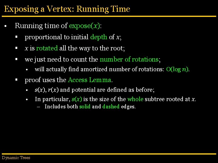
Exposing a Vertex: Running Time • Running time of expose(x): § proportional to initial depth of x; § x is rotated all the way to the root; § we just need to count the number of rotations; • § will actually find amortized number of rotations: O(log n). proof uses the Access Lemma. • s(x), r(x) and potential are defined as before; • In particular, s(x) is the size of the whole subtree rooted at x. – Includes both solid and dashed edges. Dynamic Trees

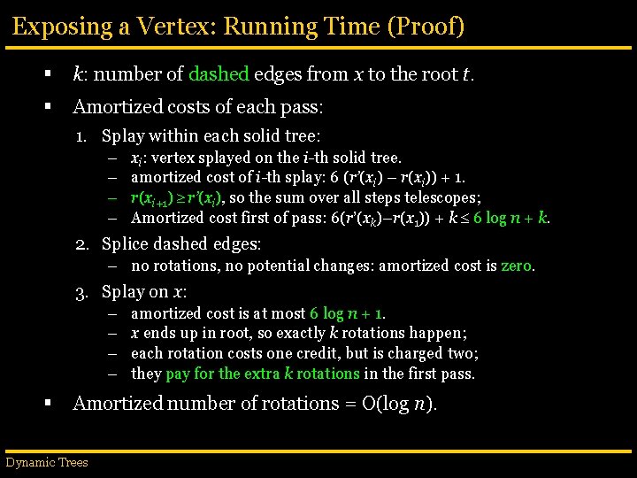
Exposing a Vertex: Running Time (Proof) § k: number of dashed edges from x to the root t. § Amortized costs of each pass: 1. Splay within each solid tree: – – xi: vertex splayed on the i-th solid tree. amortized cost of i-th splay: 6 (r’(xi) – r(xi)) + 1. r(xi+1) r’(xi), so the sum over all steps telescopes; Amortized cost first of pass: 6(r’(xk)–r(x 1)) + k 6 log n + k. 2. Splice dashed edges: – no rotations, no potential changes: amortized cost is zero. 3. Splay on x: – – § amortized cost is at most 6 log n + 1. x ends up in root, so exactly k rotations happen; each rotation costs one credit, but is charged two; they pay for the extra k rotations in the first pass. Amortized number of rotations = O(log n). Dynamic Trees

Implementing Dynamic Tree Operations • findcost(v): § expose v, return cost(v). • findroot(v): § expose v; § find w, the rightmost vertex in the solid subtree containing v; § splay at w and return w. • findmin(v): § expose v; § use cost and min to walk down from v to w, the last minimumcost node in the solid subtree; § splay at w and return w. Dynamic Trees

Implementing Dynamic Tree Operations • addcost(v, x): § expose v; § add x to cost(v); • link(v, w): § expose v and w (they are in different trees); § set p(v)=w (that is, make v a middle child of w). • cut(v): § expose v; § add cost(v) to cost(right(v)); § make p(right(v))=null and right(v)=null. Dynamic Trees

Extensions and Variants • Simple extensions: § Associate values with edges: • just interpret cost(v) as cost(v, p(v)). § other path queries (such as length): • change values stored in each node and update operations. § free (unrooted) trees. • implement evert operation, which changes the root. • Not-so-simple extension: § subtree-related operations: • requires that vertices have bounded degree; • Approach for arbitrary trees: “ternarize” them: – [Goldberg, Grigoriadis and Tarjan, 1991] Dynamic Trees

Alternative Implementation • Total time per operation depends on the data structure used to represent paths: § Splay trees: O(log n) amortized [ST 85]. § Balanced search tree: O(log 2 n) amortized [ST 83]. § Locally biased search tree: O(log n) amortized [ST 83]. § Globally biased search trees: O(log n) worst-case [ST 83]. • Biased search trees: § Support leaves with different “weights”. § Some solid leaves are “heavier” because they also represent subtrees dangling from it from dashed edges. § Much more complicated than splay trees. Dynamic Trees

Other Data Structures • Some applications require tree-related information: § minimum vertex in a tree; § add value to all elements in the tree; § link and cut as usual. • ET-Trees can do that: § Henzinger and King (1995); § Tarjan (1997). Dynamic Trees

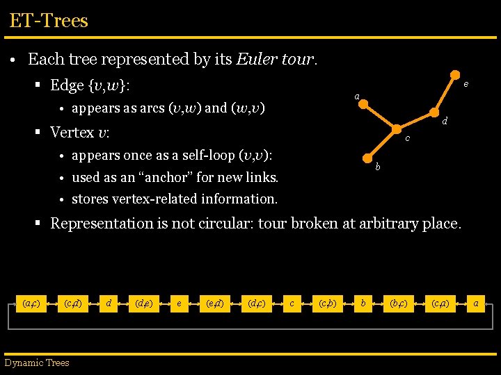
ET-Trees • Each tree represented by its Euler tour. § Edge {v, w}: e a • appears as arcs (v, w) and (w, v) d § Vertex v: c • appears once as a self-loop (v, v): b • used as an “anchor” for new links. • stores vertex-related information. § Representation is not circular: tour broken at arbitrary place. (a, c) (c, d) Dynamic Trees d (d, e) e (e, d) (d, c) c (c, b) b (b, c) (c, a) a

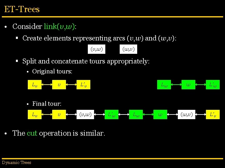
ET-Trees • Consider link(v, w): § Create elements representing arcs (v, w) and (w, v): (v, w) (w, v) § Split and concatenate tours appropriately: • Original tours: Lv v L’v Lw w L’w • Final tour: Lv v (v, w) • The cut operation is similar. Dynamic Trees L’w Lw w (w, v) L’v

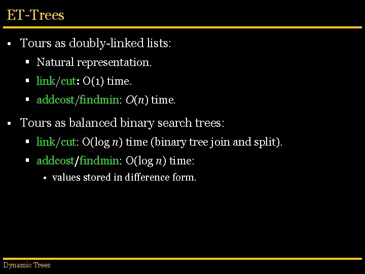
ET-Trees • Tours as doubly-linked lists: § Natural representation. § link/cut: O(1) time. § addcost/findmin: O(n) time. • Tours as balanced binary search trees: § link/cut: O(log n) time (binary tree join and split). § addcost/findmin: O(log n) time: • values stored in difference form. Dynamic Trees

Contractions • ST-Trees [ST 83, ST 85]: § first data structure to handle paths within trees efficiently. § It is clearly path-oriented: • relevant paths explicitly exposed and dealt with. • Other approaches are based on contractions: § Original tree is progressively contracted until a structure representing only the relevant path (or tree) is left. Dynamic Trees

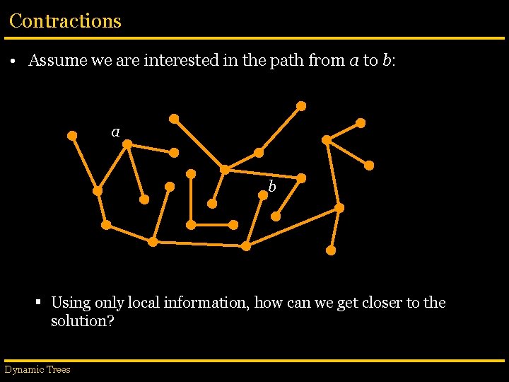
Contractions • Assume we are interested in the path from a to b: a b § Using only local information, how can we get closer to the solution? Dynamic Trees

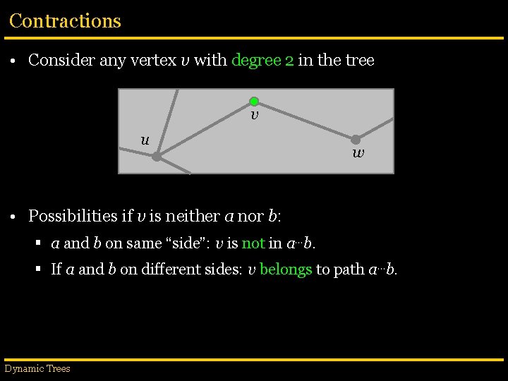
Contractions • Consider any vertex v with degree 2 in the tree v u w • Possibilities if v is neither a nor b: § a and b on same “side”: v is not in a…b. § If a and b on different sides: v belongs to path a…b. Dynamic Trees

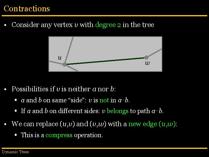
Contractions • Consider any vertex v with degree 2 in the tree u w • Possibilities if v is neither a nor b: § a and b on same “side”: v is not in a…b. § If a and b on different sides: v belongs to path a…b. • We can replace (u, v) and (v, w) with a new edge (u, w): § This is a compress operation. Dynamic Trees

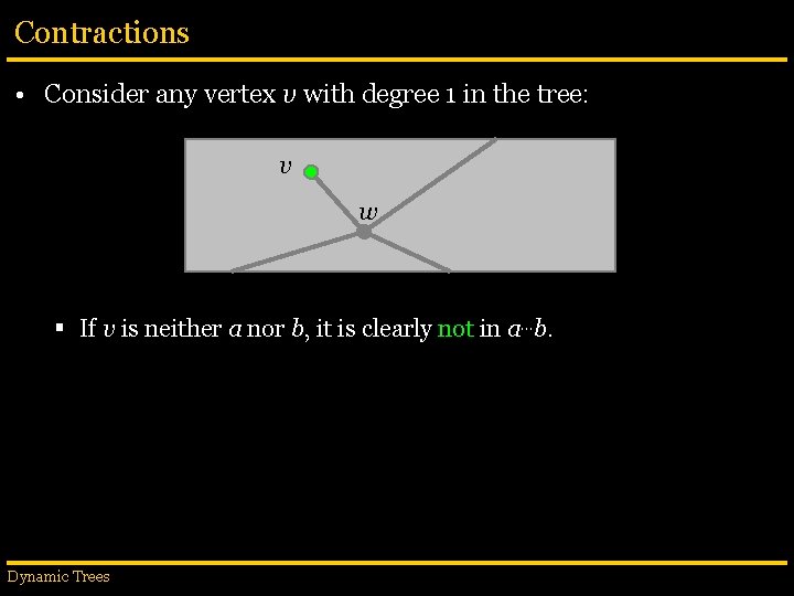
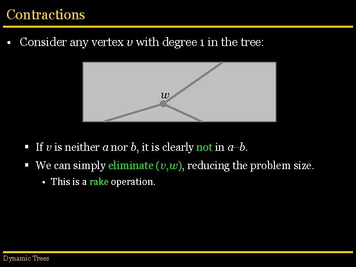
Contractions • Consider any vertex v with degree 1 in the tree: v w § If v is neither a nor b, it is clearly not in a…b. Dynamic Trees

Contractions • Consider any vertex v with degree 1 in the tree: w § If v is neither a nor b, it is clearly not in a…b. § We can simply eliminate (v, w), reducing the problem size. • This is a rake operation. Dynamic Trees

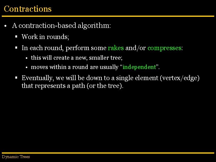
Contractions • A contraction-based algorithm: § Work in rounds; § In each round, perform some rakes and/or compresses: • this will create a new, smaller tree; • moves within a round are usually “independent”. § Eventually, we will be down to a single element (vertex/edge) that represents a path (or the tree). Dynamic Trees

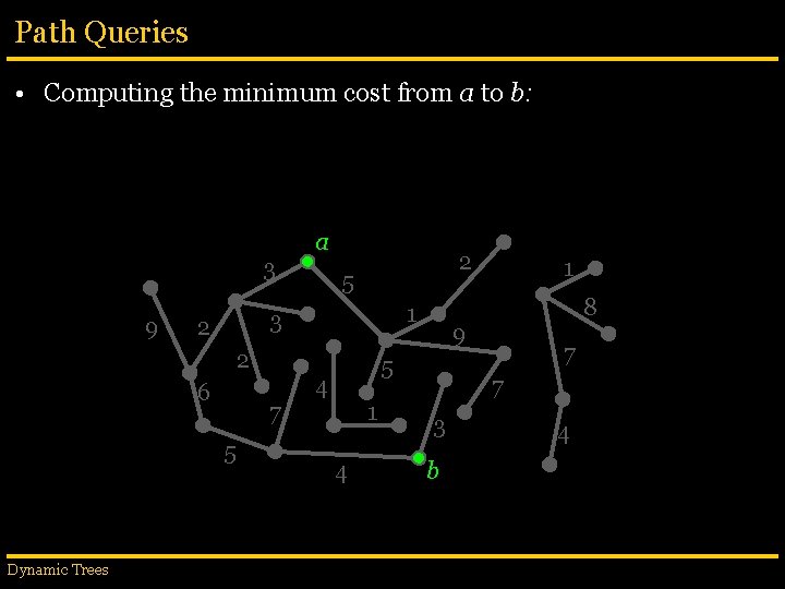
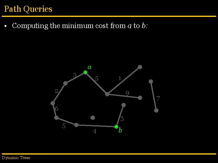
Path Queries • Computing the minimum cost from a to b: 3 9 2 5 1 3 2 2 6 7 5 Dynamic Trees a 1 4 8 9 5 4 1 7 7 3 b 4

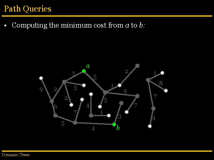
Path Queries • Computing the minimum cost from a to b: 3 9 2 5 1 3 2 2 6 7 5 Dynamic Trees a 1 4 8 9 5 4 1 7 7 3 b 4

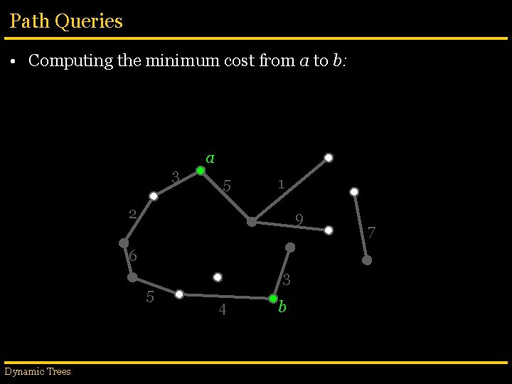
Path Queries • Computing the minimum cost from a to b: 3 a 5 1 2 9 6 5 Dynamic Trees 3 4 b 7

Path Queries • Computing the minimum cost from a to b: 3 a 5 1 2 9 6 5 Dynamic Trees 3 4 b 7

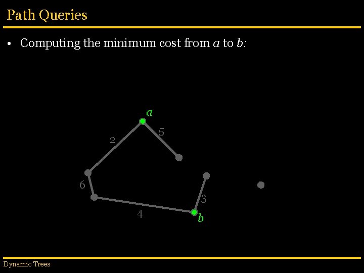
Path Queries • Computing the minimum cost from a to b: a 5 2 6 3 4 Dynamic Trees b

Path Queries • Computing the minimum cost from a to b: a 5 2 6 3 4 Dynamic Trees b

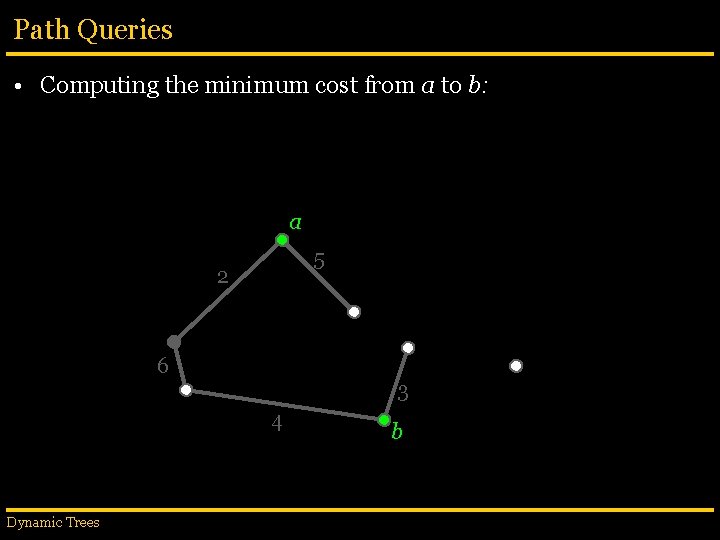
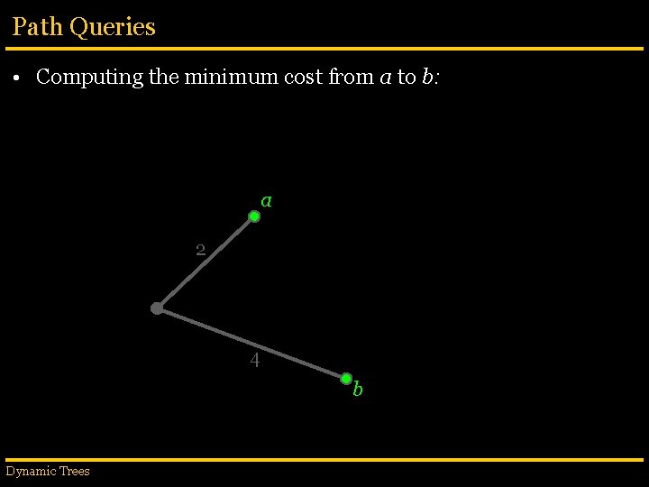
Path Queries • Computing the minimum cost from a to b: a 2 4 b Dynamic Trees

Path Queries • Computing the minimum cost from a to b: a 2 4 b Dynamic Trees

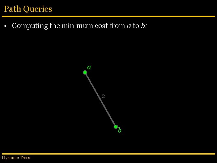
Path Queries • Computing the minimum cost from a to b: a 2 b Dynamic Trees

Contractions • Suppose a definition of independence guarantees that a fraction 1/k of all possible rakes and compresses will be executed in a round. § All degree-1 vertices are rake candidates. § All degree-2 vertices are compress candidates. § Fact: at least half the vertices in any tree have degree 1 or 2. § Result: a fraction 1/2 k of all vertices will be removed. § Total number of rounds is log(2 k)/(2 k-1)n = O(log n). Dynamic Trees

Contractions • rake and compress proposed by Miller and Reif [1985]. § Original context: parallel algorithms. § Perform several operations on trees in O(log n) time. Dynamic Trees

The Update Problem • Coming up with a definition of independence that results in a contraction with O(log n) levels. § But that is not the problem we need to solve. • Essentially, we want to repair an existing contraction after a tree operation (link/cut). • So we are interested in the update problem: § Given a contraction C of a forest F, find another contraction C’ of a forest F’ that differs from F in one single edge (inserted or deleted). § Fast: O(log n) time. Dynamic Trees

Our Problem • Several data structures deal with this problem. § [Frederickson, 85 and 97]: Topology Trees; § [Alstrup et al. , 97 and 03]: Top Trees; § [Acar et al. 03]: RC-Trees. Dynamic Trees

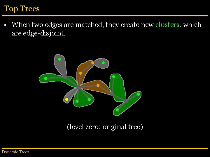
Top Trees • Proposed by Alstrup et al. [1997, 2003] • Handle unrooted (free) trees with arbitrary degrees. • Key ideas: § Associate information with the edges directly. § Pair edges up: • compress: combines two edges linked by a degree-two vertex; • rake: combines leaf with an edge with which it shares an endpoint. • All pairs (clusters) must be are disjoint. § expose: determines which two vertices are relevant to the query (they will not be raked or compressed). Dynamic Trees

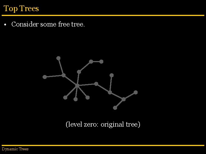
Top Trees • Consider some free tree. (level zero: original tree) Dynamic Trees

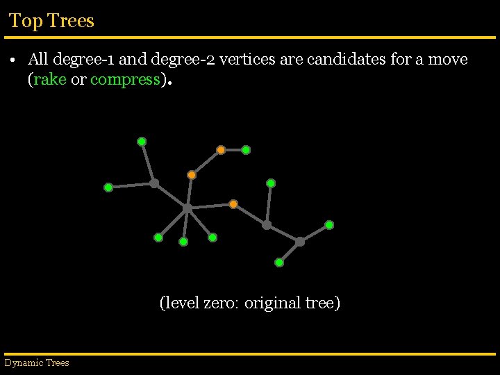
Top Trees • All degree-1 and degree-2 vertices are candidates for a move (rake or compress). (level zero: original tree) Dynamic Trees

Top Trees • When two edges are matched, they create new clusters, which are edge-disjoint. (level zero: original tree) Dynamic Trees

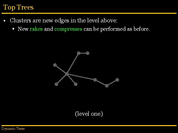
Top Trees • Clusters are new edges in the level above: § New rakes and compresses can be performed as before. (level one) Dynamic Trees

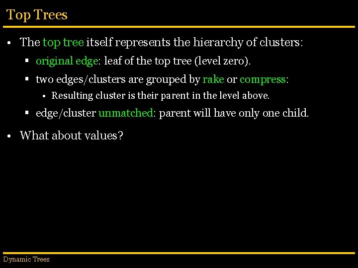
Top Trees • The top tree itself represents the hierarchy of clusters: § original edge: leaf of the top tree (level zero). § two edges/clusters are grouped by rake or compress: • Resulting cluster is their parent in the level above. § edge/cluster unmatched: parent will have only one child. • What about values? Dynamic Trees

Top Trees • Alstrup et al. see top tree as an API. • The top tree engine handles structural operations: § User has limited access to it. • Engine calls user-defined functions to handle values properly: § join(A, B, C): called when A and B are paired (by rake or compress) to create cluster C. § split(A, B, C): called when a rake or compress is undone (and C is split into A and B). § create(C, e): called when base cluster C is created to represent edge e. § destroy(C): called when base cluster C is deleted. Dynamic Trees

Top Trees • Example (path operations: findmin/addcost) § Associate two values with each cluster: • mincost(C): minimum cost in the path represented by C. • extra(C): cost that must be added to all subpaths of C. § create(C, e): (called when base cluster C is created) • mincost(C) = cost of edge e. • extra(C) = 0 § destroy(C): (called when base cluster C is deleted). • Do nothing. Dynamic Trees

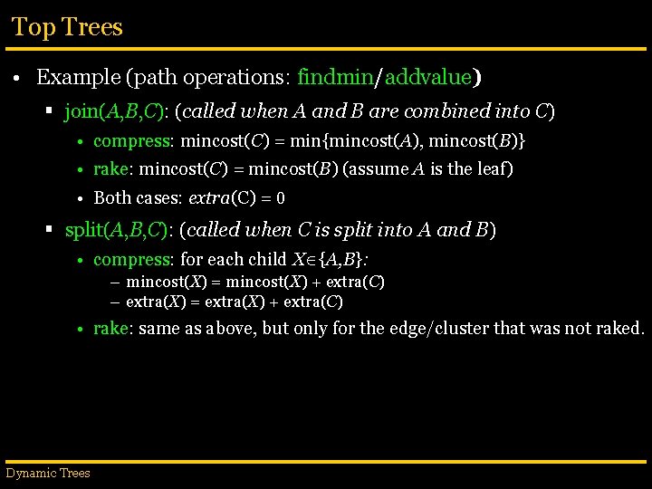
Top Trees • Example (path operations: findmin/addvalue) § join(A, B, C): (called when A and B are combined into C) • compress: mincost(C) = min{mincost(A), mincost(B)} • rake: mincost(C) = mincost(B) (assume A is the leaf) • Both cases: extra(C) = 0 § split(A, B, C): (called when C is split into A and B) • compress: for each child X {A, B}: – mincost(X) = mincost(X) + extra(C) – extra(X) = extra(X) + extra(C) • rake: same as above, but only for the edge/cluster that was not raked. Dynamic Trees

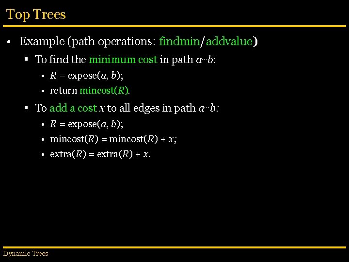
Top Trees • Example (path operations: findmin/addvalue) § To find the minimum cost in path a…b: • R = expose(a, b); • return mincost(R). § To add a cost x to all edges in path a…b: • R = expose(a, b); • mincost(R) = mincost(R) + x; • extra(R) = extra(R) + x. Dynamic Trees

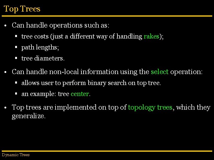
Top Trees • Can handle operations such as: § tree costs (just a different way of handling rakes); § path lengths; § tree diameters. • Can handle non-local information using the select operation: § allows user to perform binary search on top tree. § an example: tree center. • Top trees are implemented on top of topology trees, which they generalize. Dynamic Trees

Topology Trees • Proposed by Frederickson [1985, 1997]. • Work on rooted trees of bounded degree. § Assume each vertex has at most two children. • Values (and clusters) are associated with vertices. § Perform a maximal set of independent moves in each round. § Handle updates in O(log n) worst-case time. Dynamic Trees

RC-Trees • Proposed by Acar et al. [2003]. • Can be seen as a variant of topology trees. § Information stored on vertices. § Trees of bounded degree. • Main differences: § Not necessarily rooted. § Alternate rake and compress rounds. § Not maximal in compress rounds (randomization). § Updates in O(log n) expected time. Dynamic Trees

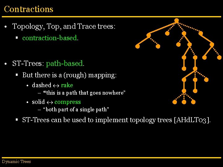
Contractions • Topology, Top, and Trace trees: § contraction-based. • ST-Trees: path-based. § But there is a (rough) mapping: • dashed rake – “this is a path that goes nowhere” • solid compress – “both part of a single path” § ST-Trees can be used to implement topology trees [AHd. LT 03]. Dynamic Trees

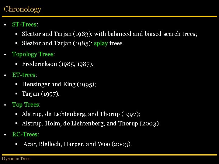
Chronology • ST-Trees: § Sleator and Tarjan (1983): with balanced and biased search trees; § Sleator and Tarjan (1985): splay trees. • Topology Trees: § Frederickson (1985, 1987). • ET-trees: § Hensinger and King (1995); § Tarjan (1997). • Top Trees: § Alstrup, de Lichtenberg, and Thorup (1997); § Alstrup, Holm, de Lichtenberg, and Thorup (2003). • RC-Trees: § Acar, Blelloch, Harper, and Woo (2003). Dynamic Trees