Trees Rooted Trees Spanning trees and Shortest Paths

Trees Rooted Trees Spanning trees and Shortest Paths 12. Graphs and Trees 2 Aaron Tan 5 – 9 November 2018 1

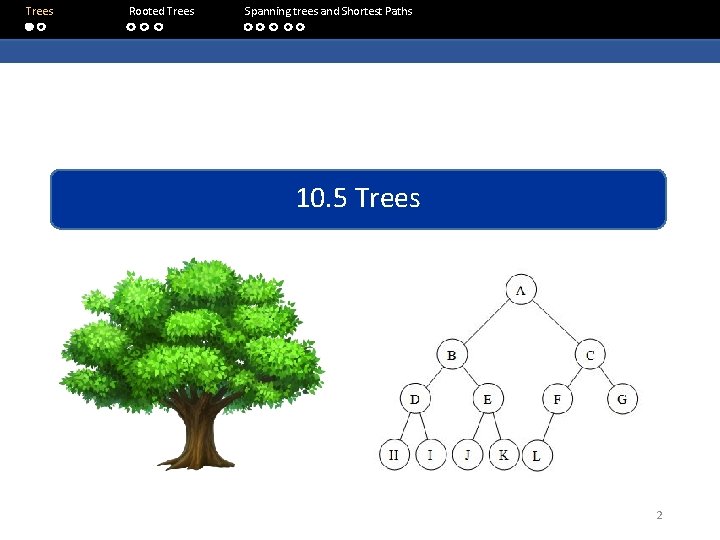
Trees Rooted Trees Spanning trees and Shortest Paths 10. 5 Trees 2

Trees Rooted Trees Spanning trees and Shortest Paths Definition: Tree A graph is said to be circuit-free if, and only if, it has no circuits. A graph is called a tree if, and only if, it is circuit-free and connected. A trivial tree is a graph that consists of a single vertex. A graph is called a forest if, and only if, it is circuit-free and not connected. 3

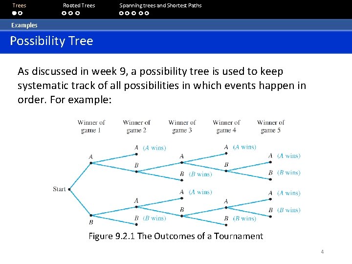
Trees Rooted Trees Spanning trees and Shortest Paths Examples Possibility Tree As discussed in week 9, a possibility tree is used to keep systematic track of all possibilities in which events happen in order. For example: Figure 9. 2. 1 The Outcomes of a Tournament 4

Trees Rooted Trees Spanning trees and Shortest Paths Examples Parse Tree In the last 30 years, Noam Chomsky and others have developed new ways to describe the syntax (or grammatical structure) of natural languages such as English. In the study of grammars, trees are often used to show the derivation of grammatically correct sentences from certain basic rules. Such trees are called syntactic derivation trees or parse trees. 5

Trees Rooted Trees Spanning trees and Shortest Paths Examples Parse Tree A very small subset of English grammar, for example, specifies that: 1. a sentence can be produced by writing first a noun phrase and then a verb phrase; 2. a noun phrase can be produced by writing an article and then a noun; 3. a noun phrase can also be produced by writing an article, then an adjective, and then a noun; 4. a verb phrase can be produced by writing a verb and then a noun phrase; 5. one article is “the”; 6. one adjective is “young”; 7. one verb is “caught”; 8. one noun is “man”; 9. one (other) noun is “ball. ” 6

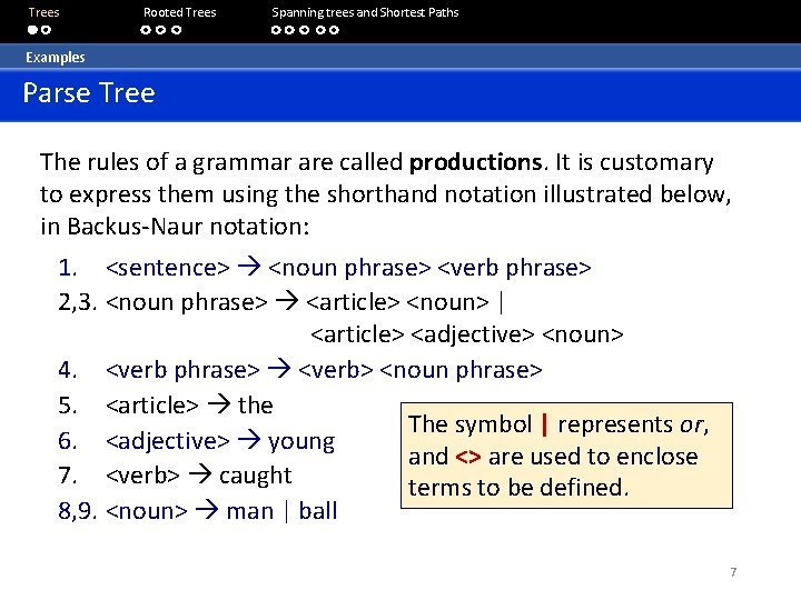
Trees Rooted Trees Spanning trees and Shortest Paths Examples Parse Tree The rules of a grammar are called productions. It is customary to express them using the shorthand notation illustrated below, in Backus-Naur notation: 1. <sentence> <noun phrase> <verb phrase> 2, 3. <noun phrase> <article> <noun> | <article> <adjective> <noun> 4. <verb phrase> <verb> <noun phrase> 5. <article> the The symbol | represents or, 6. <adjective> young and <> are used to enclose 7. <verb> caught terms to be defined. 8, 9. <noun> man | ball 7

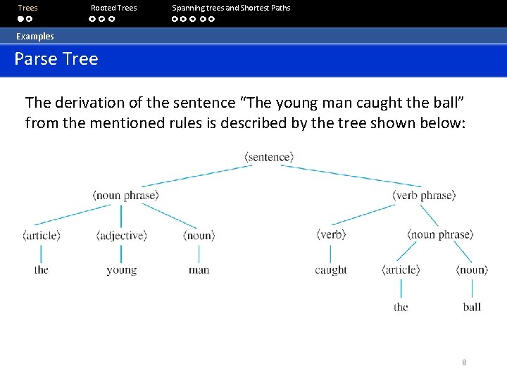
Trees Rooted Trees Spanning trees and Shortest Paths Examples Parse Tree The derivation of the sentence “The young man caught the ball” from the mentioned rules is described by the tree shown below: 8

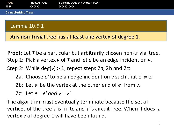
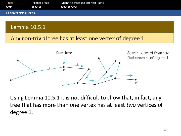
Trees Rooted Trees Spanning trees and Shortest Paths Characterizing Trees Lemma 10. 5. 1 Any non-trivial tree has at least one vertex of degree 1. Proof: Let T be a particular but arbitrarily chosen non-trivial tree. Step 1: Pick a vertex v of T and let e be an edge incident on v. Step 2: While deg(v) > 1, repeat steps 2 a, 2 b and 2 c: 2 a: Choose e' to be an edge incident on v such that e' e. 2 b: Let v' be the vertex at the other end of e' from v. 2 c: Let e = e' and v = v'. The algorithm must eventually terminate because the set of vertices of the tree T is finite and T is circuit-free. When it does, a vertex v of degree 1 will have been found. 9

Trees Rooted Trees Spanning trees and Shortest Paths Characterizing Trees Lemma 10. 5. 1 Any non-trivial tree has at least one vertex of degree 1. Using Lemma 10. 5. 1 it is not difficult to show that, in fact, any tree that has more than one vertex has at least two vertices of degree 1. 10

Trees Rooted Trees Spanning trees and Shortest Paths Characterizing Trees Definitions: Terminal vertex (leaf) and internal vertex Let T be a tree. If T has only one or two vertices, then each is called a terminal vertex (or leaf). If T has at least three vertices, then a vertex of degree 1 in T is called a terminal vertex (or leaf), and a vertex of degree greater than 1 in T is called an internal vertex. 11

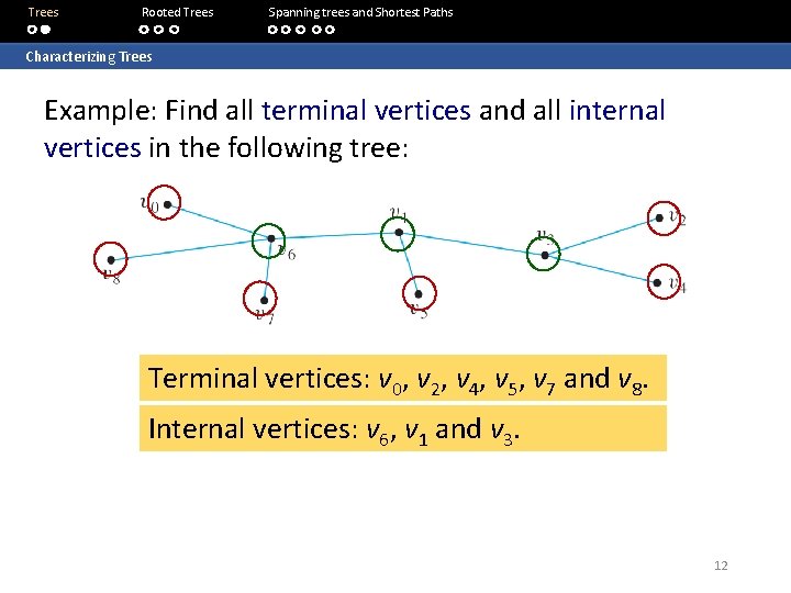
Trees Rooted Trees Spanning trees and Shortest Paths Characterizing Trees Example: Find all terminal vertices and all internal vertices in the following tree: Terminal vertices: v 0, v 2, v 4, v 5, v 7 and v 8. Internal vertices: v 6, v 1 and v 3. 12

Trees Rooted Trees Spanning trees and Shortest Paths Characterizing Trees Theorem 10. 5. 2 Any tree with n vertices (n > 0) has n – 1 edges. Proof: By mathematical induction. Let the property P(n) be “any tree with n vertices has n – 1 edges”. P(1): Let T be any tree with one vertex. Then T has no edges. So P(1) is true. Show that for all integers k 1, if P(k) is true then P(k+1) is true. Suppose P(k) is true. 1. Let T be a particular but arbitrarily chosen tree with k + 1 vertices. 2. Since k is positive, (k + 1) 2, and so T has more than one vertex. 3. Hence, by Lemma 10. 5. 1, T has a vertex v of degree 1, and has at least another vertex in T besides v. 13

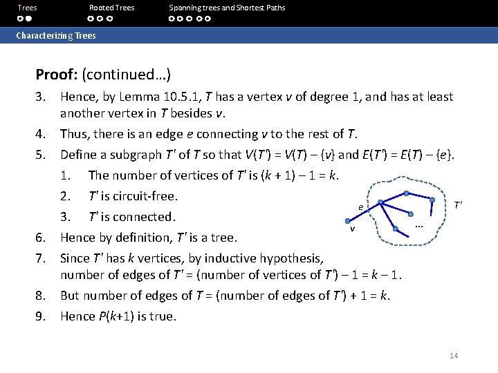
Trees Rooted Trees Spanning trees and Shortest Paths Characterizing Trees Proof: (continued…) 3. Hence, by Lemma 10. 5. 1, T has a vertex v of degree 1, and has at least another vertex in T besides v. 4. Thus, there is an edge e connecting v to the rest of T. 5. Define a subgraph T' of T so that V(T') = V(T) – {v} and E(T') = E(T) – {e}. 1. The number of vertices of T' is (k + 1) – 1 = k. 2. T' is circuit-free. T' e 3. T' is connected. … v 6. Hence by definition, T' is a tree. 7. Since T' has k vertices, by inductive hypothesis, number of edges of T' = (number of vertices of T') – 1 = k – 1. 8. But number of edges of T = (number of edges of T') + 1 = k. 9. Hence P(k+1) is true. 14

Trees Rooted Trees Spanning trees and Shortest Paths Characterizing Trees Example: Find all non-isomorphic trees with four vertices. By Theorem 10. 5. 2, any tree with four vertices has three edges. So by Theorem 10. 1. 1, the tree has a total degree of six. Also, every non-trivial tree has at least two vertices of degree 1. 15

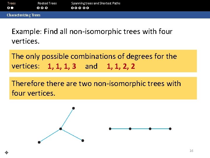
Trees Rooted Trees Spanning trees and Shortest Paths Characterizing Trees Example: Find all non-isomorphic trees with four vertices. The only possible combinations of degrees for the vertices: 1, 1, 1, 3 and 1, 1, 2, 2 Therefore there are two non-isomorphic trees with four vertices. 16

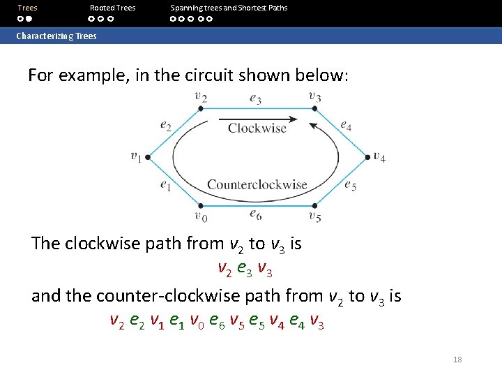
Trees Rooted Trees Spanning trees and Shortest Paths Characterizing Trees Lemma 10. 5. 3 If G is any connected graph, C is any circuit in G, and one of the edges of C is removed from G, then the graph that remains is still connected. Essentially, the reason why Lemma 10. 5. 3 is true is that any two vertices in a circuit are connected by two distinct paths. It is possible to draw the graph so that one of these goes “clockwise” and the other goes “counter-clockwise” around the circuit. 17

Trees Rooted Trees Spanning trees and Shortest Paths Characterizing Trees For example, in the circuit shown below: The clockwise path from v 2 to v 3 is v 2 e 3 v 3 and the counter-clockwise path from v 2 to v 3 is v 2 e 2 v 1 e 1 v 0 e 6 v 5 e 5 v 4 e 4 v 3 18

Trees Rooted Trees Spanning trees and Shortest Paths Characterizing Trees Theorem 10. 5. 4 If G is a connected graph with n vertices and n – 1 edges, then G is a tree. Proof: 1. Suppose G is a particular but arbitrarily chosen graph that is connected and has n vertices and n – 1 edges. 2. Since G is connected, it suffices to show that G is circuit-free. 3. Suppose G is not circuit free 1. Let C be the circuit in G. 2. By Lemma 10. 5. 3, an edge of C can be removed from G to obtain a graph G' that is connected. 3. If G' has a circuit, then repeat this process: Remove an edge of the circuit from G' to form a new connected graph. 4. Continue the process of removing edges from the circuits until eventually a graph G'' is obtained that is connected and is circuit-free. 19

Trees Rooted Trees Spanning trees and Shortest Paths Characterizing Trees Proof: (continued…) 4. Continue the process of removing edges from the circuits until eventually a graph G'' is obtained that is connected and is circuit-free. 5. By definition, G'' is a tree. 6. Since no vertices were removed from G to form G'', G'' has n vertices. 7. Thus, by Theorem 10. 5. 2, G'' has n – 1 edges. 8. But the supposition that G has a circuit implies that at least one edge of G is removed to form G''. 9. Hence G'' has no more than (n – 1) – 1 = n – 2 edges, which contradicts its having n – 1 edges. 10. So the supposition is false. 4. Hence G is circuit-free, and therefore G is a tree. 20

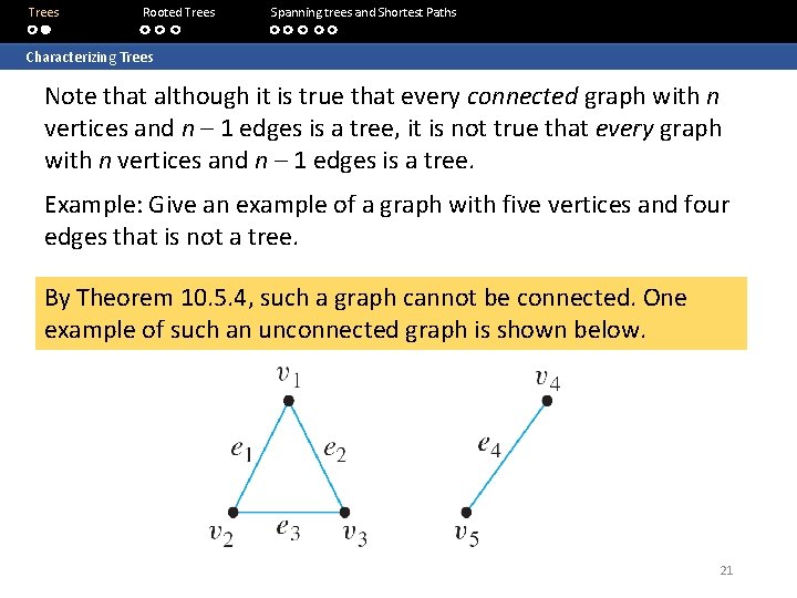
Trees Rooted Trees Spanning trees and Shortest Paths Characterizing Trees Note that although it is true that every connected graph with n vertices and n – 1 edges is a tree, it is not true that every graph with n vertices and n – 1 edges is a tree. Example: Give an example of a graph with five vertices and four edges that is not a tree. By Theorem 10. 5. 4, such a graph cannot be connected. One example of such an unconnected graph is shown below. 21

Trees Rooted Trees Spanning trees and Shortest Paths 10. 6 Rooted Trees 22

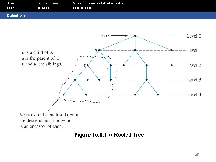
Trees Rooted Trees Spanning trees and Shortest Paths Definitions A rooted tree is a tree in which one vertex has been distinguished from the others and is designated the root. Definitions: Rooted Tree, Level, Height A rooted tree is a tree in which there is one vertex that is distinguished from the others and is called the root. The level of a vertex is the number of edges along the unique path between it and the root. The height of a rooted tree is the maximum level of any vertex of the tree. 23

Trees Rooted Trees Spanning trees and Shortest Paths Definitions: Child, Parent, Sibling, Ancestor, Descendant Given the root or any internal vertex v of a rooted tree, the children of v are all those vertices that are adjacent to v and are one level farther away from the root than v. If w is a child of v, then v is called the parent of w, and two distinct vertices that are both children of the same parent are called siblings. Given two distinct vertices v and w, if v lies on the unique path between w and the root, then v is an ancestor of w, and w is a descendant of v. 24

Trees Rooted Trees Spanning trees and Shortest Paths Definitions Figure 10. 6. 1 A Rooted Tree 25

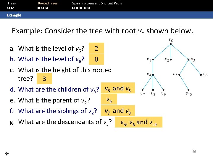
Trees Rooted Trees Spanning trees and Shortest Paths Example: Consider the tree with root v 0 shown below. a. What is the level of v 5? 2 b. What is the level of v 0? 0 c. What is the height of this rooted tree? 3 d. What are the children of v 3? v 5 and v 6 v 0 e. What is the parent of v 2? f. What are the siblings of v 8? v 7 and v 9 g. What are the descendants of v 3? v 5, v 6 and v 10 26

Trees Rooted Trees Spanning trees and Shortest Paths Binary Trees Definitions: Binary Tree, Full Binary Tree A binary tree is a rooted tree in which every parent has at most two children. Each child is designated either a left child or a right child (but not both), and every parent has at most one left child and one right child. A full binary tree is a binary tree in which each parent has exactly two children. 27

Trees Rooted Trees Spanning trees and Shortest Paths Binary Trees Definitions: Left Subtree, Right Subtree Given any parent v in a binary tree T, if v has a left child, then the left subtree of v is the binary tree whose root is the left child of v, whose vertices consist of the left child of v and all its descendants, and whose edges consist of all those edges of T that connect the vertices of the left subtree. The right subtree of v is defined analogously. 28

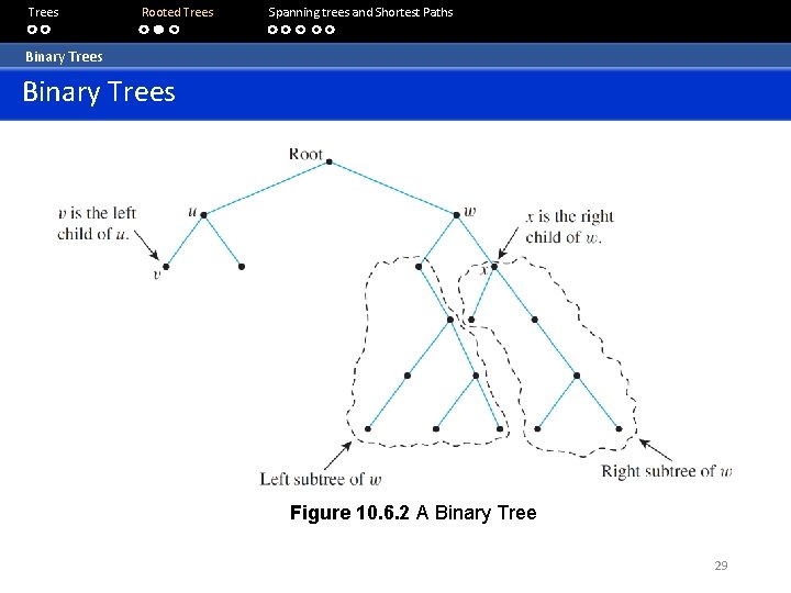
Trees Rooted Trees Spanning trees and Shortest Paths Binary Trees Figure 10. 6. 2 A Binary Tree 29

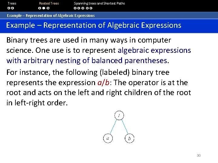
Trees Rooted Trees Spanning trees and Shortest Paths Example – Representation of Algebraic Expressions Binary trees are used in many ways in computer science. One use is to represent algebraic expressions with arbitrary nesting of balanced parentheses. For instance, the following (labeled) binary tree represents the expression a/b: The operator is at the root and acts on the left and right children of the root in left-right order. 30

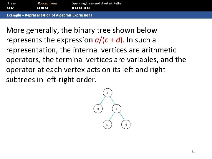
Trees Rooted Trees Spanning trees and Shortest Paths Example – Representation of Algebraic Expressions More generally, the binary tree shown below represents the expression a/(c + d). In such a representation, the internal vertices are arithmetic operators, the terminal vertices are variables, and the operator at each vertex acts on its left and right subtrees in left-right order. 31

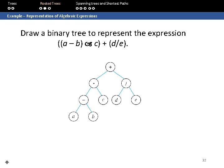
Trees Rooted Trees Spanning trees and Shortest Paths Example – Representation of Algebraic Expressions Draw a binary tree to represent the expression ((a – b) c) + (d/e). 32

Trees Rooted Trees Spanning trees and Shortest Paths Full Binary Tree An interesting theorem about binary trees says that if you know the number of internal vertices of a full binary tree, then you can calculate both the total number of vertices and the number of terminal vertices (leaves), and conversely. Theorem 10. 6. 1: Full Binary Tree Theorem If T is a full binary tree with k internal vertices, then T has a total of 2 k + 1 vertices and has k + 1 terminal vertices (leaves). 33

Trees Rooted Trees Spanning trees and Shortest Paths Full Binary Tree Proof: 1. Every vertex, except the root, has a parent. 2. Since every internal vertex of a full binary tree has exactly two children, the number of vertices that have a parent is twice the number of parents, or 2 k. #vertices of T = #vertices that have a parent + #vertices that do not have a parent = 2 k + 1 3. #terminal vertices = #vertices – #internal vertices = 2 k + 1 – k = k + 1 4. Therefore T has a total of 2 k + 1 vertices and has k + 1 terminal vertices. 34

Trees Rooted Trees Spanning trees and Shortest Paths Full Binary Tree Q: Is there a full binary tree that has 10 internal vertices and 13 terminal vertices? No, by Theorem 10. 6. 1, a full binary tree with 10 internal vertices has 10 + 1 = 11 terminal vertices. 35

Trees Rooted Trees Spanning trees and Shortest Paths Height and Terminal Vertices of a Binary Tree Theorem 10. 6. 2 For non-negative integers h, if T is any binary tree with height h and t terminal vertices (leaves), then t 2 h Equivalently, log 2 t h This theorem says that the maximum number of terminal vertices (leaves) of a binary tree of height h is 2 h. Alternatively, a binary tree with t terminal vertices (leaves) has height of at least log 2 t. 36

Trees Rooted Trees Spanning trees and Shortest Paths Height and Terminal Vertices of a Binary Tree Proof: By mathematical induction 1. Let P(h) be “If T is any binary tree of height h, then the number of leaves of T is at most 2 h. 2. P(0): T consists of one vertex, which is a terminal vertex. Hence t = 1 = 20. 3. Show that for all integers k 0, if P(i) is true for all integers i from 0 through k, then P(k+1) is true. 4. Let T be a binary tree of height k + 1, root v, and t leaves. 5. Since k 0, hence k + 1 1 and so v has at least one child. 6. We consider two cases: If v has only one child, or if v has two children. 37

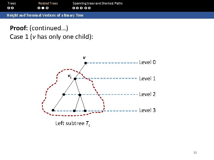
Trees Rooted Trees Spanning trees and Shortest Paths Height and Terminal Vertices of a Binary Tree Proof: (continued…) Case 1 (v has only one child): v v. L Level 0 Level 1 Level 2 Level 3 Left subtree TL 38

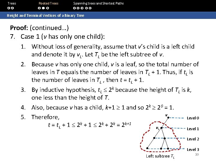
Trees Rooted Trees Spanning trees and Shortest Paths Height and Terminal Vertices of a Binary Tree Proof: (continued…) 7. Case 1 (v has only one child): 1. Without loss of generality, assume that v’s child is a left child and denote it by v. L. Let TL be the left subtree of v. 2. Because v has only one child, v is a leaf, so the total number of leaves in T equals the number of leaves in TL + 1. Thus, if t. L is the number of leaves in TL , then t = t. L + 1. 3. By inductive hypothesis, t. L 2 k because the height of TL is k, one less than the height of T. 4. Also, because v has a child, k+1 1 and so 2 k 20 = 1. v 5. Therefore, Level 0 t = t. L + 1 2 k + 2 k = 2 k+1 v. L Level 1 Level 2 Level 3 Left subtree TL 39

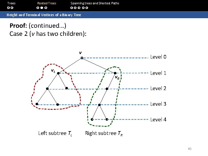
Trees Rooted Trees Spanning trees and Shortest Paths Height and Terminal Vertices of a Binary Tree Proof: (continued…) Case 2 (v has two children): v v. L Level 0 v. R Level 1 Level 2 Level 3 Level 4 Left subtree TL Right subtree TR 40

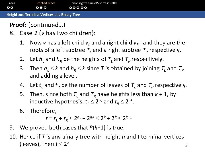
Trees Rooted Trees Spanning trees and Shortest Paths Height and Terminal Vertices of a Binary Tree Proof: (continued…) 8. Case 2 (v has two children): 1. Now v has a left child v. L and a right child v. R , and they are the roots of a left subtree TL and a right subtree TR respectively. 2. Let h. L and h. R be the heights of TL and TR respectively. 3. Then h. L k and h. R k since T is obtained by joining TL and TR and adding a level. 4. Let t. L and t. R be the number of leaves of TL and TR respectively. 5. Then, since both TL and TR have heights less than k + 1, by inductive hypothesis, t. L 2 h. L and t. R 2 h. R. 6. Therefore, t = t. L + t. R 2 h. L + 2 h. R 2 k + 2 k 2 k+1 9. We proved both cases that P(k+1) is true. 10. Hence if T is any binary tree with height h and t terminal vertices (leaves), then t 2 h. 41

Trees Rooted Trees Spanning trees and Shortest Paths Height and Terminal Vertices of a Binary Tree Q: Is there a binary tree that has height 5 and 38 terminal vertices? No, by Theorem 10. 6. 2, any binary tree T with height 5 has at most 25 = 32 terminal vertices, so such a tree cannot have 38 terminal vertices. 42

Trees Rooted Trees Spanning trees and Shortest Paths Binary Tree Traversal Tree traversal (also known as tree search) is the process of visiting each node in a tree data structure exactly once in a systematic manner. There are two types of traversal: breadth-first search (BFS) or depth-first search (DFS). The following sections describe BFS and DFS on binary trees, but in general they can be applied on any type of trees, or even graphs. 43

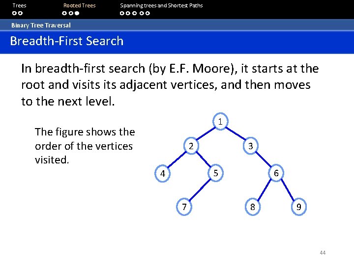
Trees Rooted Trees Spanning trees and Shortest Paths Binary Tree Traversal Breadth-First Search In breadth-first search (by E. F. Moore), it starts at the root and visits adjacent vertices, and then moves to the next level. 1 The figure shows the order of the vertices visited. 2 3 5 4 7 6 8 9 44

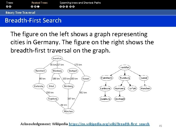
Trees Rooted Trees Spanning trees and Shortest Paths Binary Tree Traversal Breadth-First Search The figure on the left shows a graph representing cities in Germany. The figure on the right shows the breadth-first traversal on the graph. Acknowledgement: Wikipedia https: //en. wikipedia. org/wiki/Breadth-first_search 45

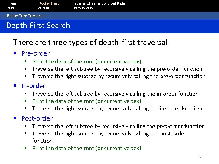
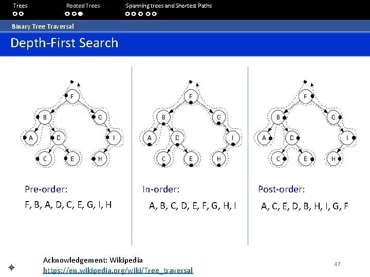
Trees Rooted Trees Spanning trees and Shortest Paths Binary Tree Traversal Depth-First Search There are three types of depth-first traversal: § Pre-order § Print the data of the root (or current vertex) § Traverse the left subtree by recursively calling the pre-order function § Traverse the right subtree by recursively calling the pre-order function § In-order § Traverse the left subtree by recursively calling the in-order function § Print the data of the root (or current vertex) § Traverse the right subtree by recursively calling the in-order function § Post-order § Traverse the left subtree by recursively calling the post-order function § Traverse the right subtree by recursively calling the post-order function § Print the data of the root (or current vertex) 46

Trees Rooted Trees Spanning trees and Shortest Paths Binary Tree Traversal Depth-First Search Pre-order: F, B, A, D, C, E, G, I, H In-order: A, B, C, D, E, F, G, H, I Acknowledgement: Wikipedia https: //en. wikipedia. org/wiki/Tree_traversal Post-order: A, C, E, D, B, H, I, G, F 47

Trees Rooted Trees Spanning trees and Shortest Paths 10. 7 Spanning Trees and Shortest Paths 48

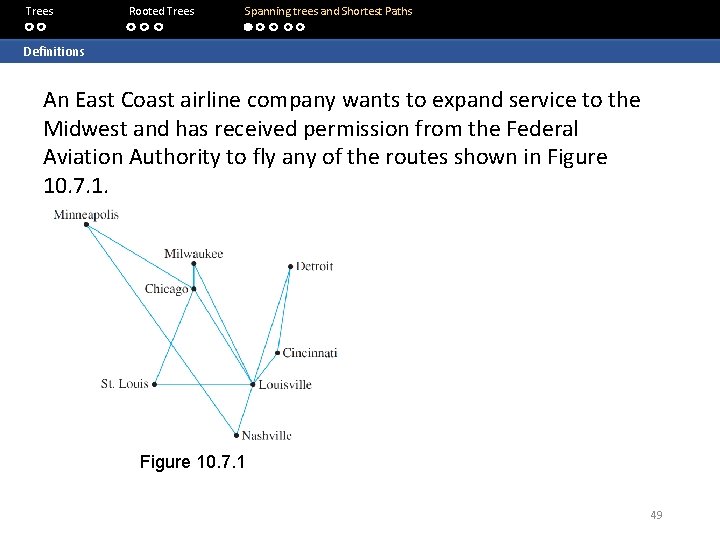
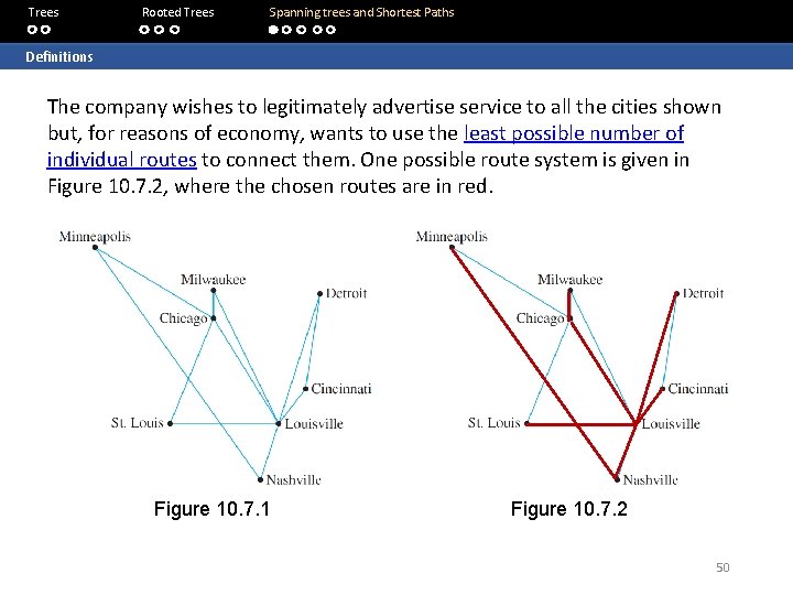
Trees Rooted Trees Spanning trees and Shortest Paths Definitions An East Coast airline company wants to expand service to the Midwest and has received permission from the Federal Aviation Authority to fly any of the routes shown in Figure 10. 7. 1 49

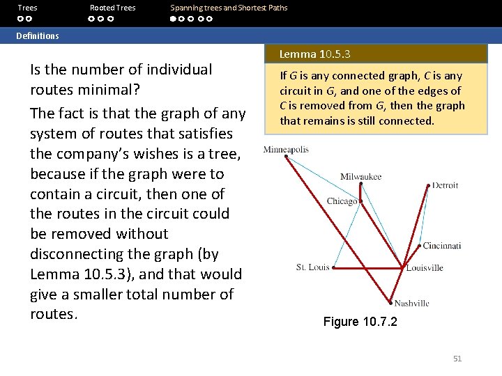
Trees Rooted Trees Spanning trees and Shortest Paths Definitions The company wishes to legitimately advertise service to all the cities shown but, for reasons of economy, wants to use the least possible number of individual routes to connect them. One possible route system is given in Figure 10. 7. 2, where the chosen routes are in red. Figure 10. 7. 1 Figure 10. 7. 2 50

Trees Rooted Trees Spanning trees and Shortest Paths Definitions Is the number of individual routes minimal? The fact is that the graph of any system of routes that satisfies the company’s wishes is a tree, because if the graph were to contain a circuit, then one of the routes in the circuit could be removed without disconnecting the graph (by Lemma 10. 5. 3), and that would give a smaller total number of routes. Lemma 10. 5. 3 If G is any connected graph, C is any circuit in G, and one of the edges of C is removed from G, then the graph that remains is still connected. Figure 10. 7. 2 51

Trees Rooted Trees Spanning trees and Shortest Paths Definitions What you have seen is a spanning tree. Definition: Spanning Tree A spanning tree for a graph G is a subgraph of G that contains every vertex of G and is a tree. Proposition 10. 7. 1 1. Every connected graph has a spanning tree. 2. Any two spanning trees for a graph have the same number of edges. 52

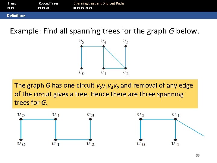
Trees Rooted Trees Spanning trees and Shortest Paths Definitions Example: Find all spanning trees for the graph G below. The graph G has one circuit v 2 v 1 v 4 v 2 and removal of any edge of the circuit gives a tree. Hence there are three spanning trees for G. 53

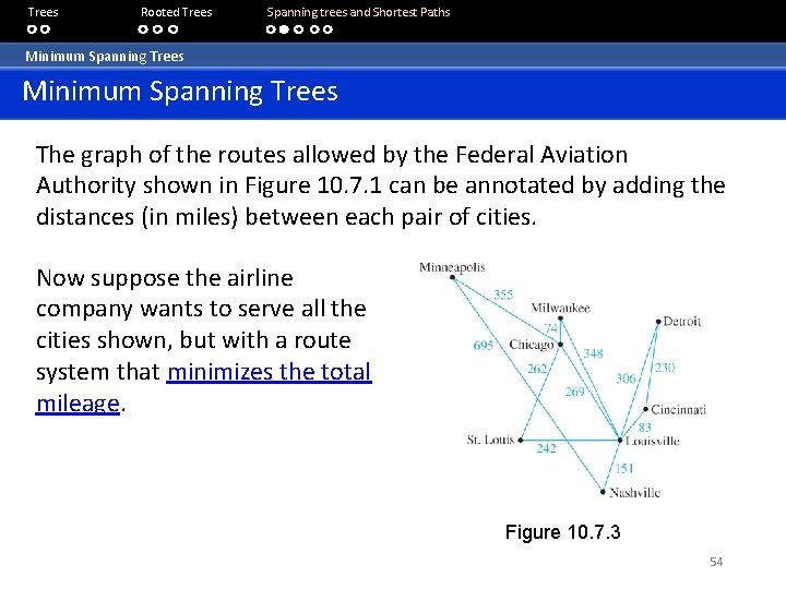
Trees Rooted Trees Spanning trees and Shortest Paths Minimum Spanning Trees The graph of the routes allowed by the Federal Aviation Authority shown in Figure 10. 7. 1 can be annotated by adding the distances (in miles) between each pair of cities. Now suppose the airline company wants to serve all the cities shown, but with a route system that minimizes the total mileage. Figure 10. 7. 3 54

Trees Rooted Trees Spanning trees and Shortest Paths Minimum Spanning Trees Definitions: Weighted Graph, Minimum Spanning Tree A weighted graph is a graph for which each edge has an associated positive real number weight. The sum of the weights of all the edges is the total weight of the graph. A minimum spanning tree for a connected weighted graph is a spanning tree that has the least possible total weight compared to all other spanning trees for the graph. If G is a weighted graph and e is an edge of G, then w(e) denotes the weight of e and w(G) denotes the total weight of G. 55

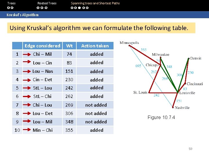
Trees Rooted Trees Spanning trees and Shortest Paths Kruskal’s Algorithm (Joseph B. Kruskal, 1956) In Kruskal’s algorithm, the edges of a connected weighted graph are examined one by one in order of increasing weight. At each stage the edge being examined is added to what will become the minimum spanning tree, provided that this addition does not create a circuit. After n – 1 edges have been added (where n is the number of vertices of the graph), these edges, together with the vertices of the graph, form a minimum spanning tree for the graph. 56

Trees Rooted Trees Spanning trees and Shortest Paths Kruskal’s Algorithm 10. 7. 1 Kruskal Input: G [a connected weighted graph with n vertices] Algorithm: 1. Initialize T to have all the vertices of G and no edges. 2. Let E be the set of all edges of G, and let m = 0. 3. While (m < n – 1) 3 a. Find an edge e in E of least weight. 3 b. Delete e from E. 3 c. If addition of e to the edge set of T does not produce a circuit, then add e to the edge set of T and set m = m + 1 End while Output: T [T is a minimum spanning tree for G] 57

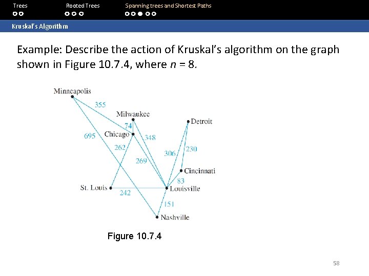
Trees Rooted Trees Spanning trees and Shortest Paths Kruskal’s Algorithm Example: Describe the action of Kruskal’s algorithm on the graph shown in Figure 10. 7. 4, where n = 8. Figure 10. 7. 4 58

Trees Rooted Trees Spanning trees and Shortest Paths Kruskal’s Algorithm Using Kruskal’s algorithm we can formulate the following table. Edge considered Wt Action taken 1 Chi – Mil 74 added 2 Lou – Cin 83 added 3 Lou – Nas 151 added 4 Cin – Det 230 5 St. L – Lou 242 added 6 St. L – Chi 262 added 7 Chi – Lou 269 not added 8 Lou – Det 306 not added 9 Lou – Mil 348 not added 10 Min – Chi 355 added Figure 10. 7. 4 59

Trees Rooted Trees Spanning trees and Shortest Paths Kruskal’s Algorithm When Kruskal’s algorithm is used on a graph in which some edges have the same weight as others, more than one minimum spanning tree can occur as output. To make the output unique, the edges of the graph can be placed in an array and edges having the same weight can be added in the order they appear in the array. 60

Trees Rooted Trees Spanning trees and Shortest Paths Prim’s Algorithm (Robert C. Prim, 1957) Prim’s algorithm works differently from Kruskal’s. It builds a minimum spanning tree T by expanding outward in connected links from some vertex. One edge and one vertex are added at each stage. The edge added is the one of least weight that connects the vertices already in T with those not in T, and the vertex is the endpoint of this edge that is not already in T. 61

Trees Rooted Trees Spanning trees and Shortest Paths Prim’s Algorithm 10. 7. 2 Prim Input: G [a connected weighted graph with n vertices] Algorithm: 1. Pick a vertex v of G and let T be the graph with this vertex only. 2. Let V be the set of all vertices of G except v. 3. For i = 1 to n – 1 3 a. Find an edge e of G such that (1) e connects T to one of the vertices in V, and (2) e has the least weight of all edges connecting T to a vertex in V. Let w be the endpoint of e that is in V. 3 b. Add e and w to the edge and vertex sets of T, and delete w from V. Output: T [T is a minimum spanning tree for G] 62

Trees Rooted Trees Spanning trees and Shortest Paths Prim’s Algorithm Example: Describe the action of Prim’s algorithm on the graph shown in Figure 10. 7. 6, using the Minneapolis vertex as a starting point. Figure 10. 7. 6 63

Trees Rooted Trees Spanning trees and Shortest Paths Prim’s Algorithm Using Prim’s algorithm we can formulate the following table. Vertex added Edge added Weight 0 Minneapolis 1 Chicago Min – Chi 355 2 Milwaukee Chi – Mil 74 3 St. Louis Chi – St. L 262 4 Louisville St. L – Lou 242 5 Cincinnati Lou – Cin 83 6 Nashville Lou – Nas 151 7 Detroit Cin – Det 230 Figure 10. 7. 6 64

Trees Rooted Trees Spanning trees and Shortest Paths Prim’s Algorithm Note that the tree obtained is the same as that obtained by Kruskal’s algorithm, but the edges are added in a different order. As with Kruskal’s algorithm, in order to ensure a unique output, the edges of the graph could be placed in an array and those with the same weight could be added in the order they appear in the array. 65

Trees Rooted Trees Spanning trees and Shortest Paths Dijkstra’s Shortest Path Algorithm Note that Dijkstra’s Shortest Path Algorithm is taken out of the curriculum this semester. However, the slides are retained here for your own reading. To skip slides 67 till end. 66

Trees Rooted Trees Spanning trees and Shortest Paths Dijkstra’s Shortest Path Algorithm In 1959, Edsgar Dijkstra developed an algorithm to find the shortest path between a starting vertex (source) and an ending vertex (destination) in a weighted graph in which all weights are positive. Somewhat similar to Prim’s algorithms, it works outward from the source a, adding vertices and edges one by one to construct a shortest path tree T. It differs from Prim’s algorithm in the way it chooses the next vertex to add, ensuring that for each added vertex v, the length of the shortest path from a to v has been identified. 67

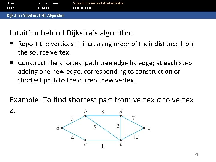
Trees Rooted Trees Spanning trees and Shortest Paths Dijkstra’s Shortest Path Algorithm Intuition behind Dijkstra’s algorithm: § Report the vertices in increasing order of their distance from the source vertex. § Construct the shortest path tree edge by edge; at each step adding one new edge, corresponding to construction of shortest path to the current new vertex. Example: To find shortest part from vertex a to vertex z. 1 68

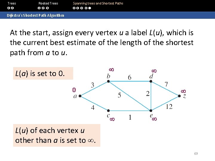
Trees Rooted Trees Spanning trees and Shortest Paths Dijkstra’s Shortest Path Algorithm At the start, assign every vertex u a label L(u), which is the current best estimate of the length of the shortest path from a to u. L(a) is set to 0. 0 1 L(u) of each vertex u other than a is set to . 69

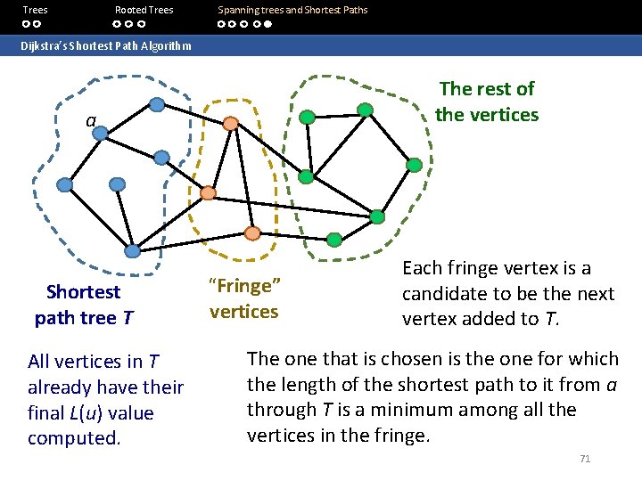
Trees Rooted Trees Spanning trees and Shortest Paths Dijkstra’s Shortest Path Algorithm As the algorithm progresses, the values of L(u) are updated, eventually becoming the actual lengths of the shortest paths from a to u. We construct the shortest path tree T outward from a. At each stage of the algorithm, the only vertices that are candidates to join T are those that are adjacent to at least one vertex of T. We call these candidates the set of “fringe” vertices. The graph G can be thought of as divided into 3 parts: the tree T that is being built up, the set of “fringe” vertices, and the rest of the vertices in G. 70

Trees Rooted Trees Spanning trees and Shortest Paths Dijkstra’s Shortest Path Algorithm The rest of the vertices a Shortest path tree T All vertices in T already have their final L(u) value computed. “Fringe” vertices Each fringe vertex is a candidate to be the next vertex added to T. The one that is chosen is the one for which the length of the shortest path to it from a through T is a minimum among all the vertices in the fringe. 71

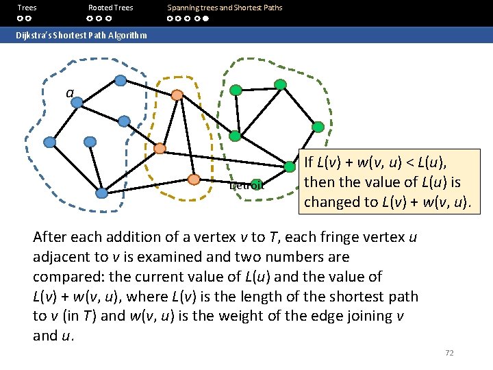
Trees Rooted Trees Spanning trees and Shortest Paths Dijkstra’s Shortest Path Algorithm a Detroit If L(v) + w(v, u) < L(u), then the value of L(u) is changed to L(v) + w(v, u). After each addition of a vertex v to T, each fringe vertex u adjacent to v is examined and two numbers are compared: the current value of L(u) and the value of L(v) + w(v, u), where L(v) is the length of the shortest path to v (in T ) and w(v, u) is the weight of the edge joining v and u. 72

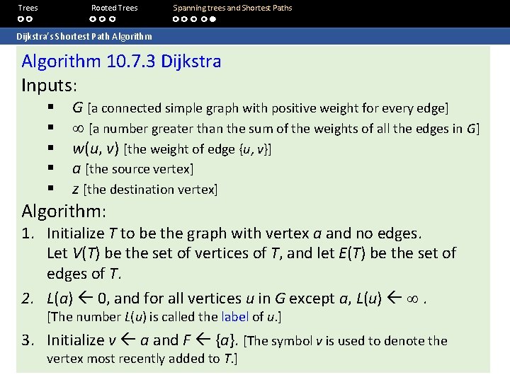
Trees Rooted Trees Spanning trees and Shortest Paths Dijkstra’s Shortest Path Algorithm 10. 7. 3 Dijkstra Inputs: § § § G [a connected simple graph with positive weight for every edge] [a number greater than the sum of the weights of all the edges in G] w(u, v) [the weight of edge {u, v}] a [the source vertex] z [the destination vertex] Algorithm: 1. Initialize T to be the graph with vertex a and no edges. Let V(T) be the set of vertices of T, and let E(T) be the set of edges of T. 2. L(a) 0, and for all vertices u in G except a, L(u) . [The number L(u) is called the label of u. ] 3. Initialize v a and F {a}. [The symbol v is used to denote the vertex most recently added to T. ] 73

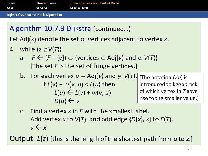
Trees Rooted Trees Spanning trees and Shortest Paths Dijkstra’s Shortest Path Algorithm 10. 7. 3 Dijkstra (continued…) Let Adj(x) denote the set of vertices adjacent to vertex x. 4. while (z V(T)) a. F (F – {v}) {vertices Adj(v) and V(T)} [The set F is the set of fringe vertices. ] b. For each vertex u Adj(v) and V(T), [The notation D(u) is introduced to keep track if L(v) + w(v, u) < L(u) then of which vertex in T gave L(u) L(v) + w(v, u) rise to the smaller value. ] D(u) v c. Find a vertex x in F with the smallest label. Add vertex x to V(T), and add edge {D(x), x} to E(T). v x Output: L(z) [this is the length of the shortest path from a to z. ] 74

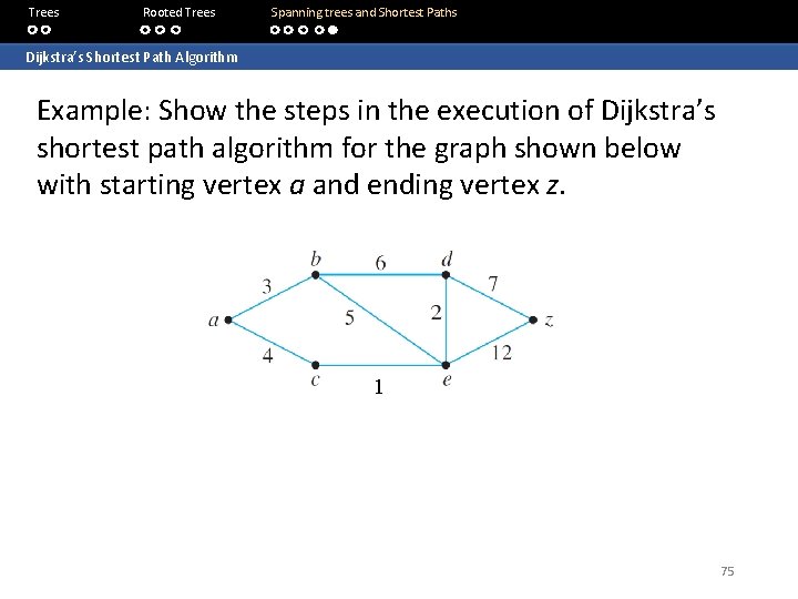
Trees Rooted Trees Spanning trees and Shortest Paths Dijkstra’s Shortest Path Algorithm Example: Show the steps in the execution of Dijkstra’s shortest path algorithm for the graph shown below with starting vertex a and ending vertex z. 1 75

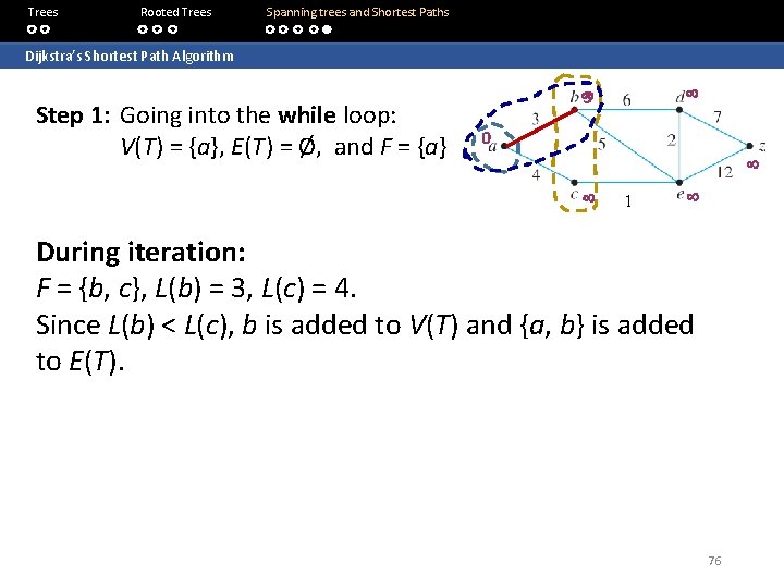
Trees Rooted Trees Spanning trees and Shortest Paths Dijkstra’s Shortest Path Algorithm Step 1: Going into the while loop: V(T ) = {a}, E(T ) = Ø, and F = {a} 3 0 1 During iteration: F = {b, c}, L(b) = 3, L(c) = 4. Since L(b) < L(c), b is added to V(T) and {a, b} is added to E(T). 76

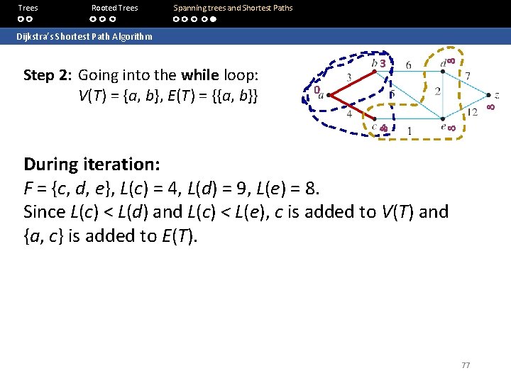
Trees Rooted Trees Spanning trees and Shortest Paths Dijkstra’s Shortest Path Algorithm Step 2: Going into the while loop: V(T ) = {a, b}, E(T ) = {{a, b}} 3 0 4 1 During iteration: F = {c, d, e}, L(c) = 4, L(d) = 9, L(e) = 8. Since L(c) < L(d) and L(c) < L(e), c is added to V(T) and {a, c} is added to E(T). 77

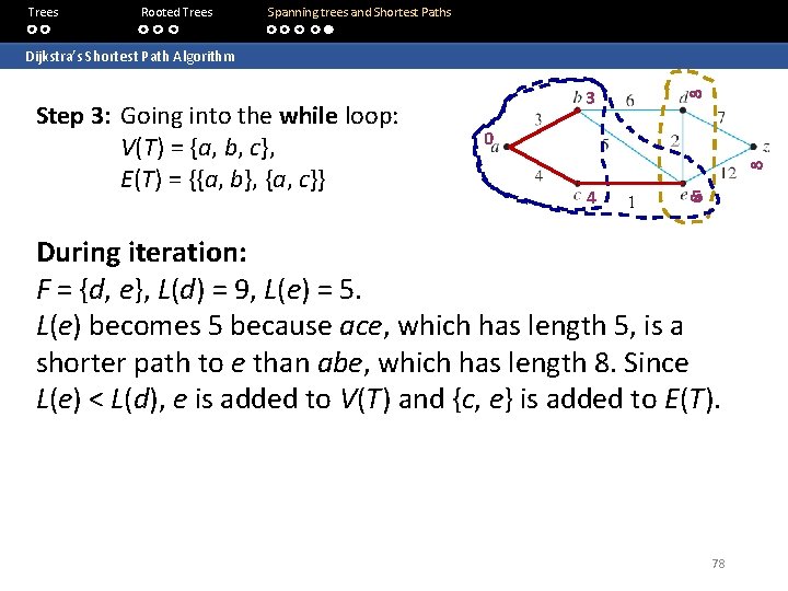
Trees Rooted Trees Spanning trees and Shortest Paths Dijkstra’s Shortest Path Algorithm Step 3: Going into the while loop: V(T ) = {a, b, c}, E(T ) = {{a, b}, {a, c}} 3 0 4 1 5 During iteration: F = {d, e}, L(d) = 9, L(e) = 5. L(e) becomes 5 because ace, which has length 5, is a shorter path to e than abe, which has length 8. Since L(e) < L(d), e is added to V(T ) and {c, e} is added to E(T ). 78

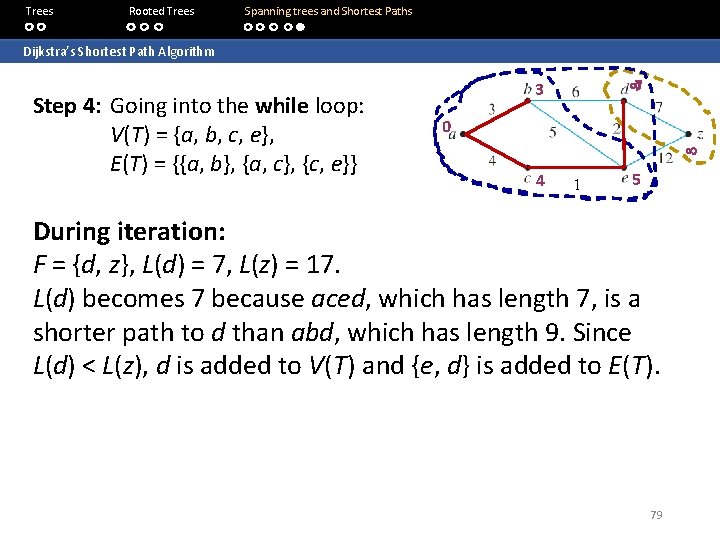
Trees Rooted Trees Spanning trees and Shortest Paths Dijkstra’s Shortest Path Algorithm Step 4: Going into the while loop: V(T ) = {a, b, c, e}, E(T ) = {{a, b}, {a, c}, {c, e}} 7 3 0 4 1 5 During iteration: F = {d, z}, L(d) = 7, L(z) = 17. L(d) becomes 7 because aced, which has length 7, is a shorter path to d than abd, which has length 9. Since L(d) < L(z), d is added to V(T ) and {e, d} is added to E(T ). 79

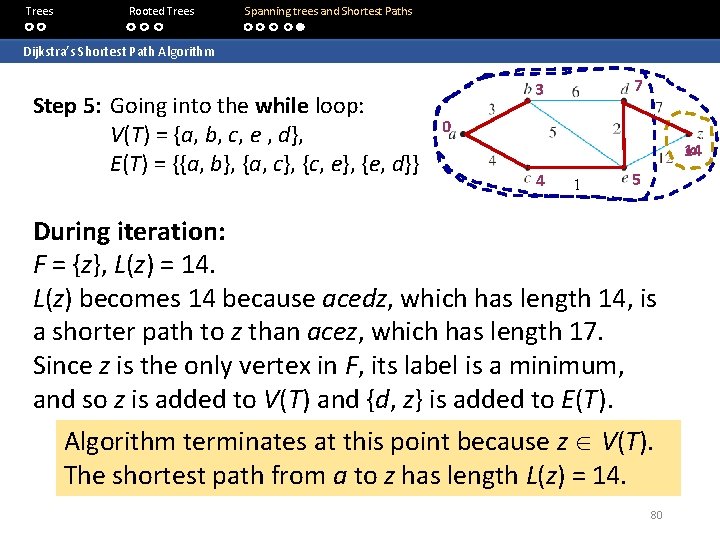
Trees Rooted Trees Spanning trees and Shortest Paths Dijkstra’s Shortest Path Algorithm Step 5: Going into the while loop: V(T ) = {a, b, c, e , d}, E(T ) = {{a, b}, {a, c}, {c, e}, {e, d}} 7 3 0 14 4 1 5 During iteration: F = {z}, L(z) = 14. L(z) becomes 14 because acedz, which has length 14, is a shorter path to z than acez, which has length 17. Since z is the only vertex in F, its label is a minimum, and so z is added to V(T ) and {d, z} is added to E(T ). Algorithm terminates at this point because z V(T). The shortest path from a to z has length L(z) = 14. 80

Trees Rooted Trees Spanning trees and Shortest Paths Dijkstra’s Shortest Path Algorithm Keeping track of the steps in a table is a convenient way to show the action of Dijkstra’s algorithm. Table 10. 7. 1 does this for the graph in the previous example. {d, z}} Table 10. 7. 1 81

END OF FILE 82