Data Structures Week 6 Special Trees Borahan Tmer

Data Structures – Week #6 Special Trees Borahan Tümer, Ph. D.

Outline • Adelson-Velskii-Landis (AVL) Trees • Splay Trees • B-Trees 2/21/2021 Borahan Tümer, Ph. D. 2

AVL Trees 2/21/2021 Borahan Tümer, Ph. D. 3

Motivation for AVL Trees • Accessing a node in a BST takes O(log 2 n) in average. • A BST can be structured so as to have an average access time of O(n). Can you think of one such BST? • Q: Is there a way to guarantee a worst-case access time of O(log 2 n) per node or can we find a way to guarantee a BST depth of O(log 2 n)? • A: AVL Trees 2/21/2021 Borahan Tümer, Ph. D. 4

Definition An AVL tree is a BST with the following balance condition: for each node in the BST, the height of left and right sub-trees can differ by at most 1, or 2/21/2021 Borahan Tümer, Ph. D. 5

Remarks on Balance Condition • Balance condition must be easy to maintain: – This is the reason, for example, for the balance condition’s not being as follows: the height of left and right sub-trees of each node have the same height. • It ensures the depth of the BST is O(log 2 n). • The height information is stored as an additional field in BTNode. Type. 2/21/2021 Borahan Tümer, Ph. D. 6

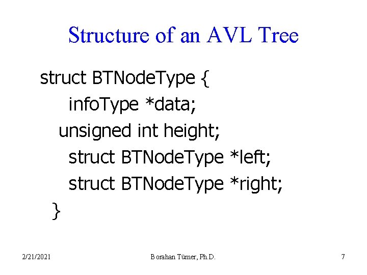
Structure of an AVL Tree struct BTNode. Type { info. Type *data; unsigned int height; struct BTNode. Type *left; struct BTNode. Type *right; } 2/21/2021 Borahan Tümer, Ph. D. 7

Rotations Definition: • Rotation is the operation performed on a BST to restore its AVL property lost as a result of an insert operation. • We consider the node whose new balance violates the AVL condition. 2/21/2021 Borahan Tümer, Ph. D. 8

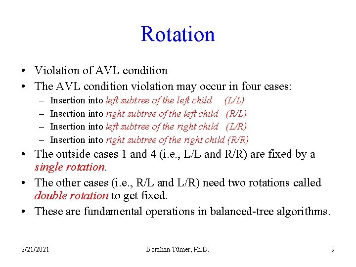
Rotation • Violation of AVL condition • The AVL condition violation may occur in four cases: – – Insertion into left subtree of the left child (L/L) Insertion into right subtree of the left child (R/L) Insertion into left subtree of the right child (L/R) Insertion into right subtree of the right child (R/R) • The outside cases 1 and 4 (i. e. , L/L and R/R) are fixed by a single rotation. • The other cases (i. e. , R/L and L/R) need two rotations called double rotation to get fixed. • These are fundamental operations in balanced-tree algorithms. 2/21/2021 Borahan Tümer, Ph. D. 9

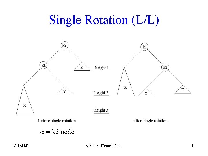
Single Rotation (L/L) k 2 node 2/21/2021 Borahan Tümer, Ph. D. 10

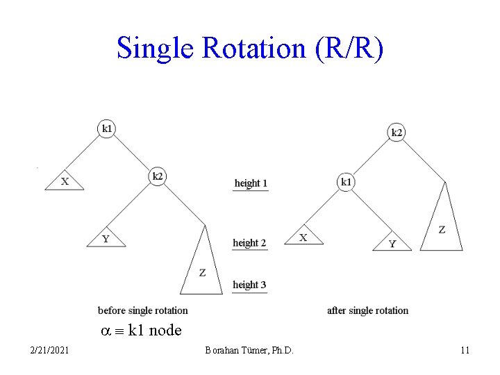
Single Rotation (R/R) k 1 node 2/21/2021 Borahan Tümer, Ph. D. 11

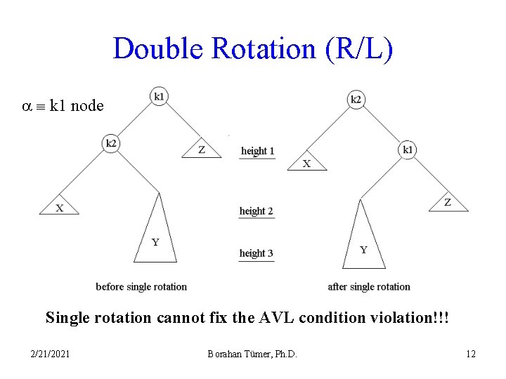
Double Rotation (R/L) k 1 node Single rotation cannot fix the AVL condition violation!!! 2/21/2021 Borahan Tümer, Ph. D. 12

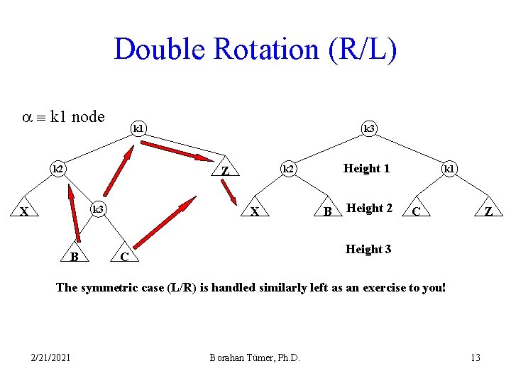
Double Rotation (R/L) k 1 node k 1 k 2 k 3 X B Height 1 k 2 Z X B Height 2 k 1 Z C Height 3 C The symmetric case (L/R) is handled similarly left as an exercise to you! 2/21/2021 Borahan Tümer, Ph. D. 13

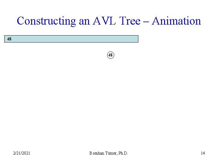
Constructing an AVL Tree – Animation 48 48 2/21/2021 Borahan Tümer, Ph. D. 14

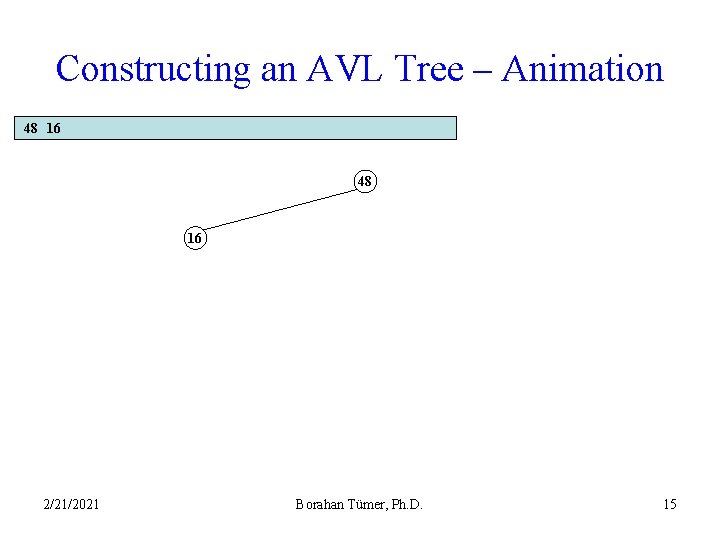
Constructing an AVL Tree – Animation 48 16 2/21/2021 Borahan Tümer, Ph. D. 15

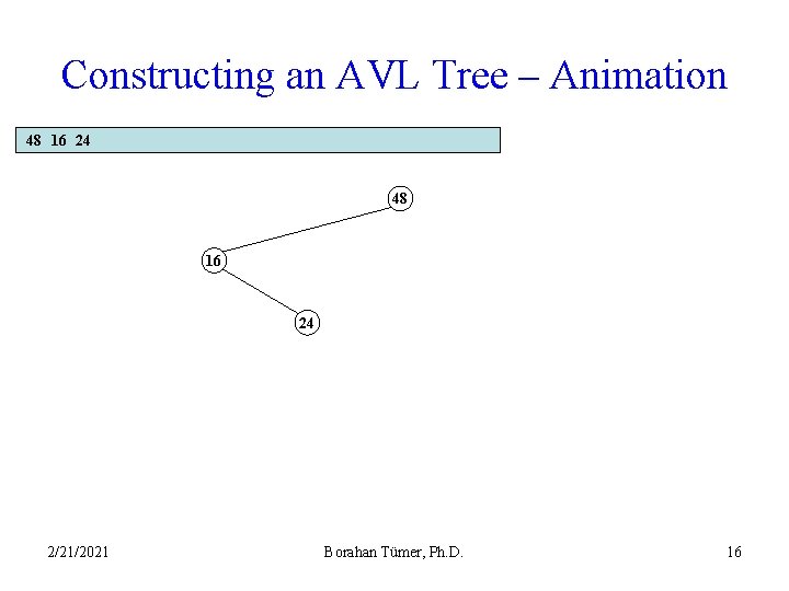
Constructing an AVL Tree – Animation 48 16 24 2/21/2021 Borahan Tümer, Ph. D. 16

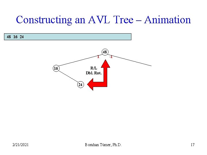
Constructing an AVL Tree – Animation 48 16 24 48 1 -1 R/L Dbl. Rot. 16 24 2/21/2021 Borahan Tümer, Ph. D. 17

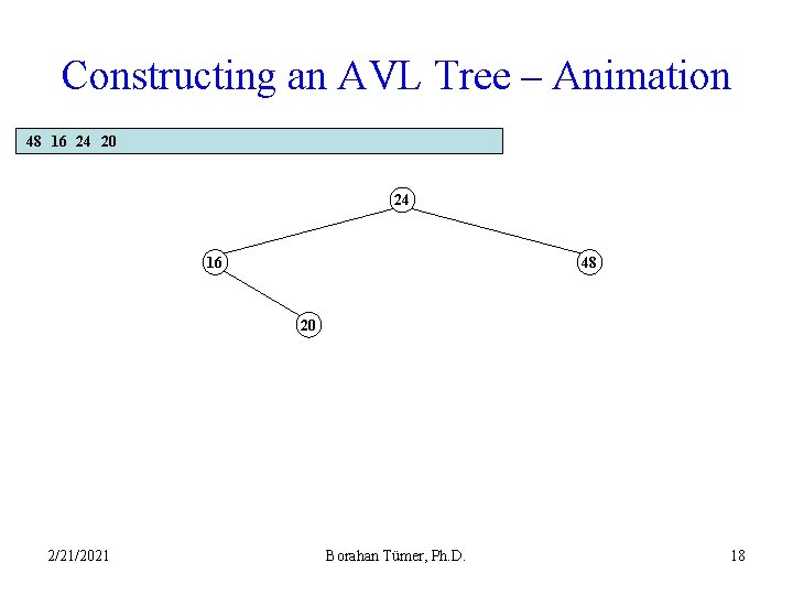
Constructing an AVL Tree – Animation 48 16 24 20 24 16 48 20 2/21/2021 Borahan Tümer, Ph. D. 18

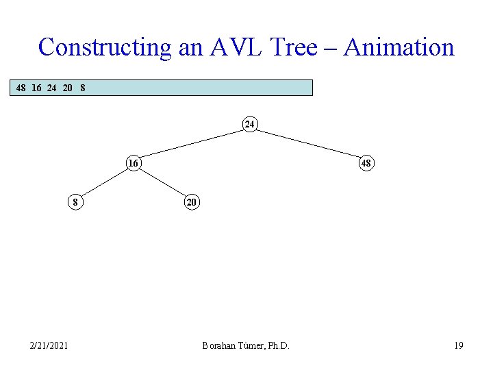
Constructing an AVL Tree – Animation 48 16 24 20 8 24 16 8 2/21/2021 48 20 Borahan Tümer, Ph. D. 19

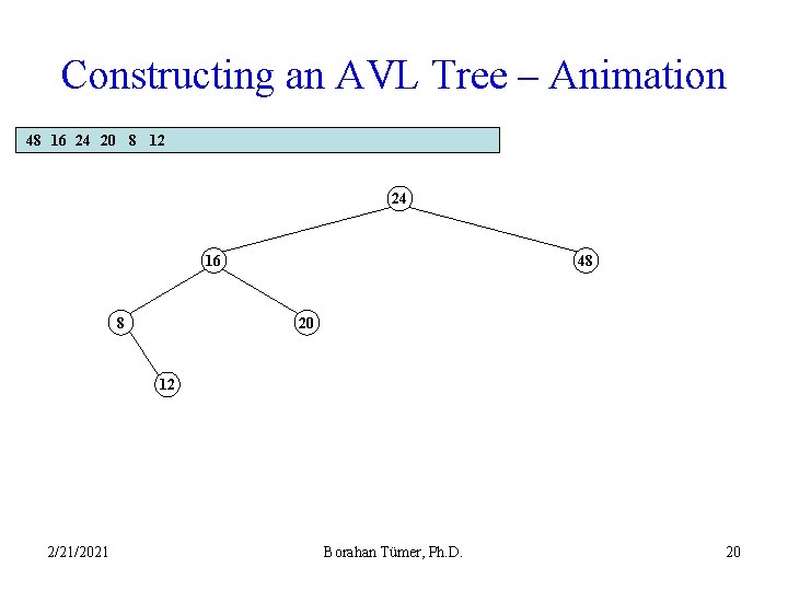
Constructing an AVL Tree – Animation 48 16 24 20 8 12 24 16 8 48 20 12 2/21/2021 Borahan Tümer, Ph. D. 20

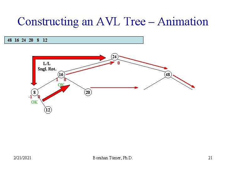
Constructing an AVL Tree – Animation 48 16 24 20 8 12 24 2 L/L Sngl. Rot. 0 16 48 1 0 OK 8 20 -1 0 OK 12 2/21/2021 Borahan Tümer, Ph. D. 21

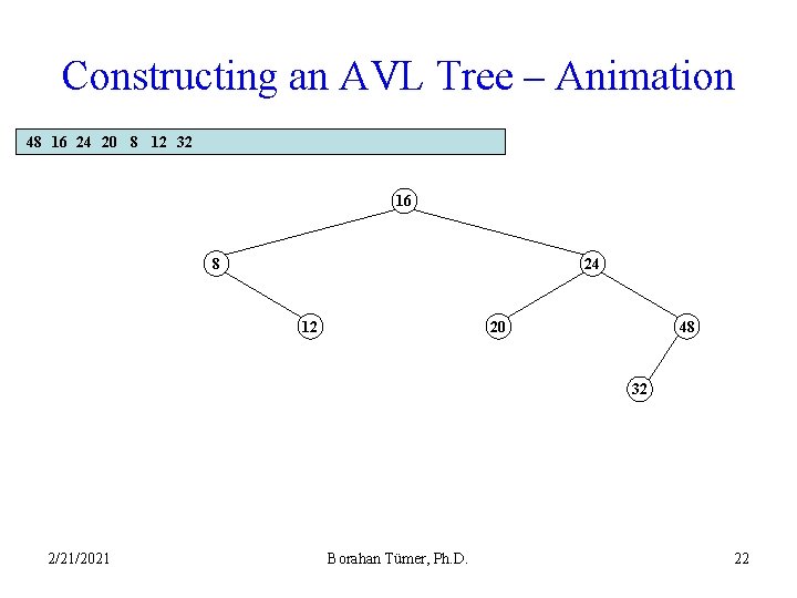
Constructing an AVL Tree – Animation 48 16 24 20 8 12 32 16 8 24 12 20 48 32 2/21/2021 Borahan Tümer, Ph. D. 22

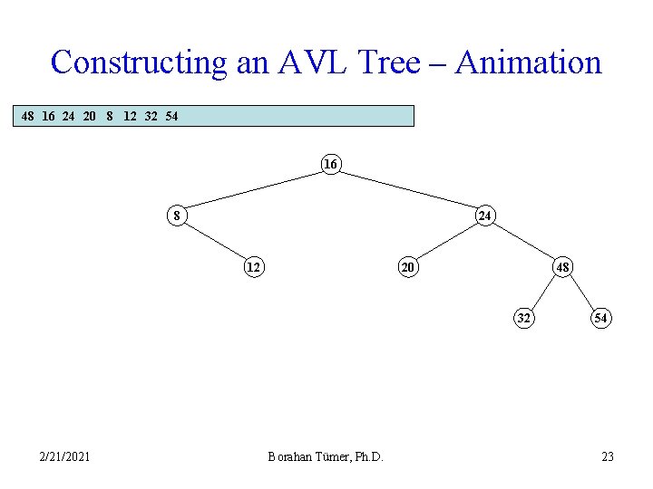
Constructing an AVL Tree – Animation 48 16 24 20 8 12 32 54 16 8 24 12 20 48 32 2/21/2021 Borahan Tümer, Ph. D. 54 23

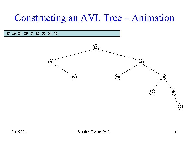
Constructing an AVL Tree – Animation 48 16 24 20 8 12 32 54 72 16 8 24 12 20 48 32 54 72 2/21/2021 Borahan Tümer, Ph. D. 24

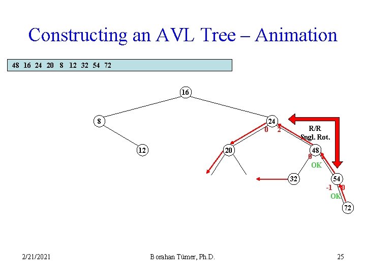
Constructing an AVL Tree – Animation 48 16 24 20 8 12 32 54 72 16 8 24 0 12 R/R Sngl. Rot. 2 20 48 0 1 OK 32 54 -1 0 OK 72 2/21/2021 Borahan Tümer, Ph. D. 25

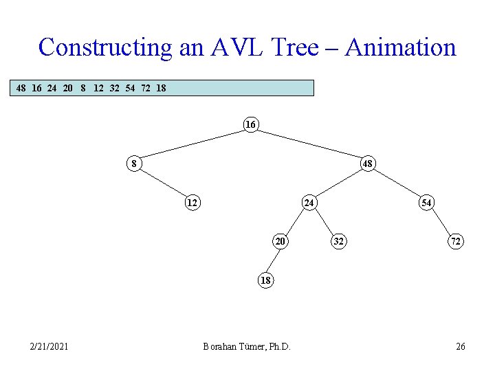
Constructing an AVL Tree – Animation 48 16 24 20 8 12 32 54 72 18 16 8 48 12 24 20 54 32 72 18 2/21/2021 Borahan Tümer, Ph. D. 26

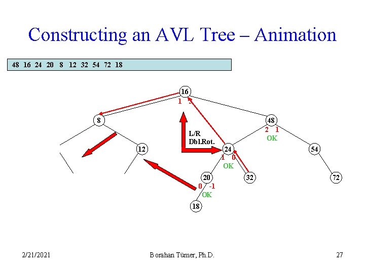
Constructing an AVL Tree – Animation 48 16 24 20 8 12 32 54 72 18 16 1 3 8 12 L/R Dbl. Rot. 20 0 -1 OK 48 2 1 OK 24 1 0 OK 54 32 72 18 2/21/2021 Borahan Tümer, Ph. D. 27

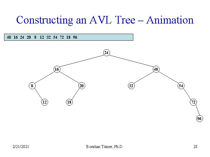
Constructing an AVL Tree – Animation 48 16 24 20 8 12 32 54 72 18 96 24 16 48 20 8 12 32 18 54 72 96 2/21/2021 Borahan Tümer, Ph. D. 28

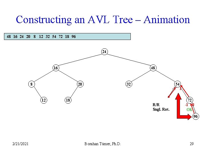
Constructing an AVL Tree – Animation 48 16 24 20 8 12 32 54 72 18 96 24 16 48 20 8 12 32 18 54 -1 1 R/R Sngl. Rot. 72 -1 0 OK 96 2/21/2021 Borahan Tümer, Ph. D. 29

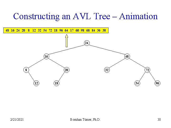
Constructing an AVL Tree – Animation 48 16 24 20 8 12 32 54 72 18 96 64 17 60 98 68 84 36 30 24 16 48 20 8 12 2/21/2021 32 18 72 54 Borahan Tümer, Ph. D. 96 30

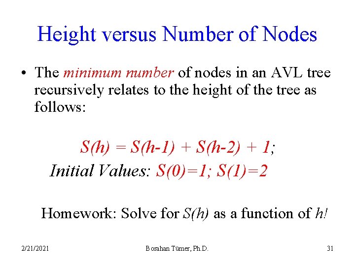
Height versus Number of Nodes • The minimum number of nodes in an AVL tree recursively relates to the height of the tree as follows: S(h) = S(h-1) + S(h-2) + 1; Initial Values: S(0)=1; S(1)=2 Homework: Solve for S(h) as a function of h! 2/21/2021 Borahan Tümer, Ph. D. 31

Splay Trees 2/21/2021 Borahan Tümer, Ph. D. 32

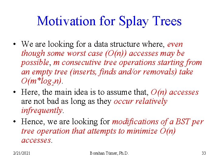
Motivation for Splay Trees • We are looking for a data structure where, even though some worst case (O(n)) accesses may be possible, m consecutive tree operations starting from an empty tree (inserts, finds and/or removals) take O(m*log 2 n). • Here, the main idea is to assume that, O(n) accesses are not bad as long as they occur relatively infrequently. • Hence, we are looking for modifications of a BST per tree operation that attempts to minimize O(n) accesses. 2/21/2021 Borahan Tümer, Ph. D. 33

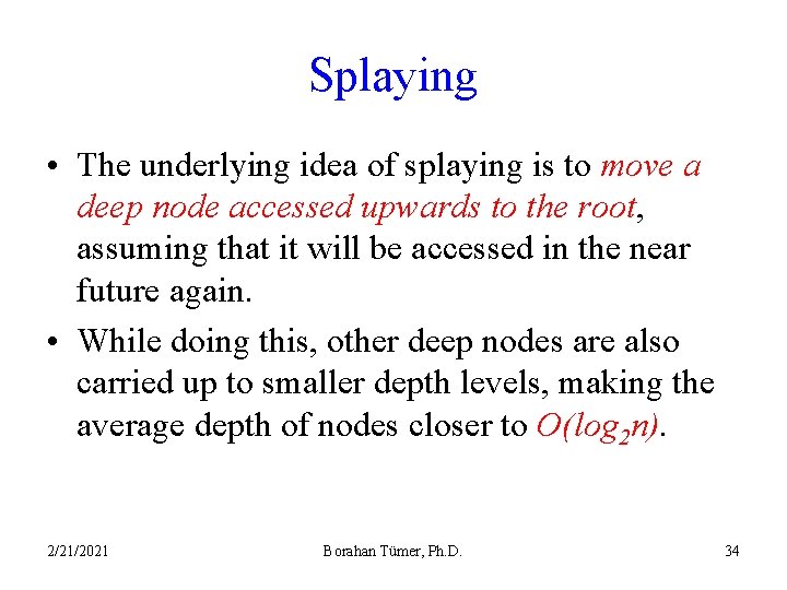
Splaying • The underlying idea of splaying is to move a deep node accessed upwards to the root, assuming that it will be accessed in the near future again. • While doing this, other deep nodes are also carried up to smaller depth levels, making the average depth of nodes closer to O(log 2 n). 2/21/2021 Borahan Tümer, Ph. D. 34

Splaying • Splaying is similar to bottom-up AVL rotations • If a node X is the child of the root R, – then we rotate only X and R, and this is the last rotation performed. else consider X, its parent P and grandparent G. Two cases and their symmetries to consider Zig-zag case, and Zig-zig case. 2/21/2021 Borahan Tümer, Ph. D. 35

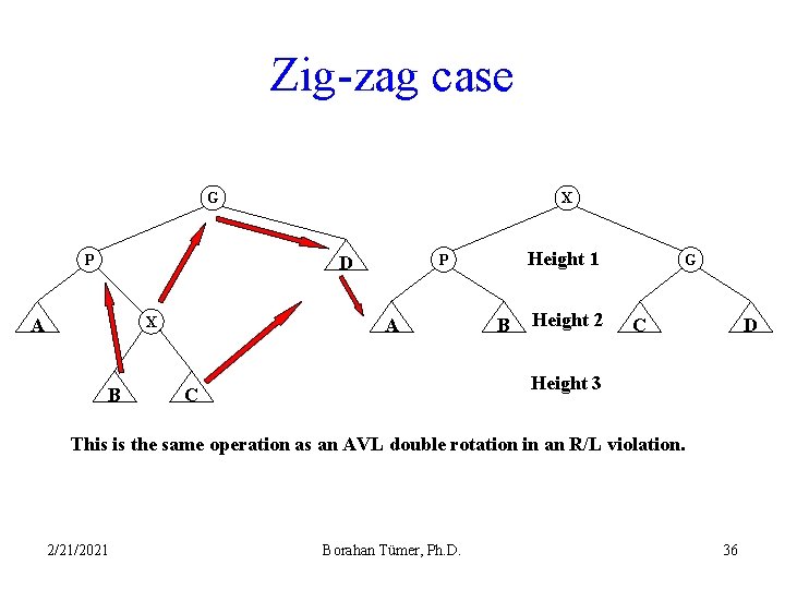
Zig-zag case G P X X A B Height 1 P D A B Height 2 G D C Height 3 C This is the same operation as an AVL double rotation in an R/L violation. 2/21/2021 Borahan Tümer, Ph. D. 36

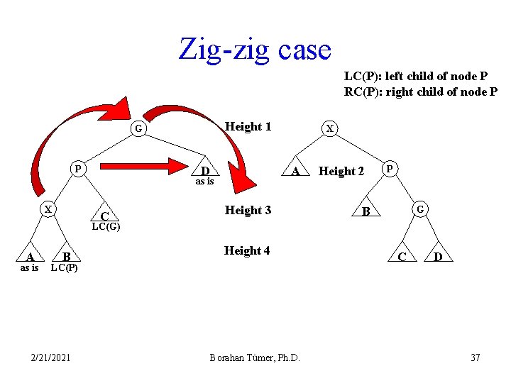
Zig-zig case LC(P): left child of node P RC(P): right child of node P Height 1 G P D A as is X C X Height 3 Height 2 P G B LC(G) A as is B Height 4 LC(P) 2/21/2021 Borahan Tümer, Ph. D. C D 37

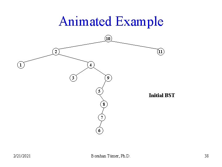
Animated Example 10 2 11 1 4 3 9 5 Initial BST 8 7 6 2/21/2021 Borahan Tümer, Ph. D. 38

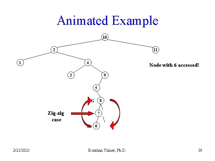
Animated Example 10 2 11 1 4 Node with 6 accessed! 3 9 5 8 G Zig-zig case X 2/21/2021 7 P 6 Borahan Tümer, Ph. D. 39

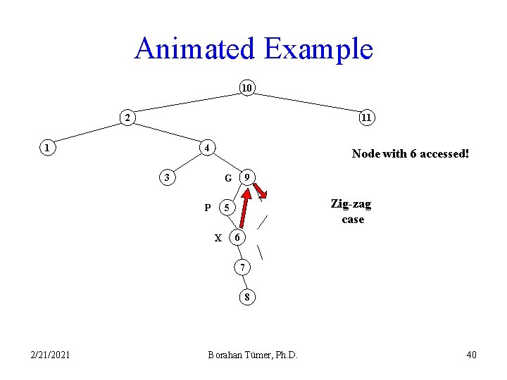
Animated Example 10 2 11 1 4 Node with 6 accessed! 3 9 G Zig-zag case 5 P X 6 7 8 2/21/2021 Borahan Tümer, Ph. D. 40

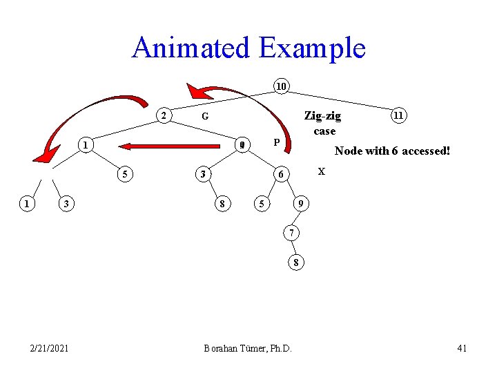
Animated Example 10 2 1 1 3 P 94 5 Zig-zig case G 73 Node with 6 accessed! X 6 8 11 5 9 7 8 2/21/2021 Borahan Tümer, Ph. D. 41

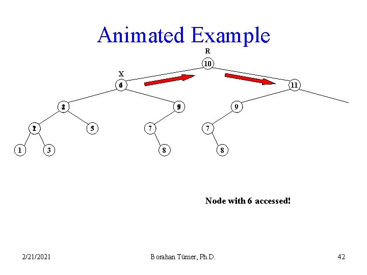
Animated Example R 10 X 46 11 24 12 1 59 35 3 7 9 7 8 8 Node with 6 accessed! 2/21/2021 Borahan Tümer, Ph. D. 42

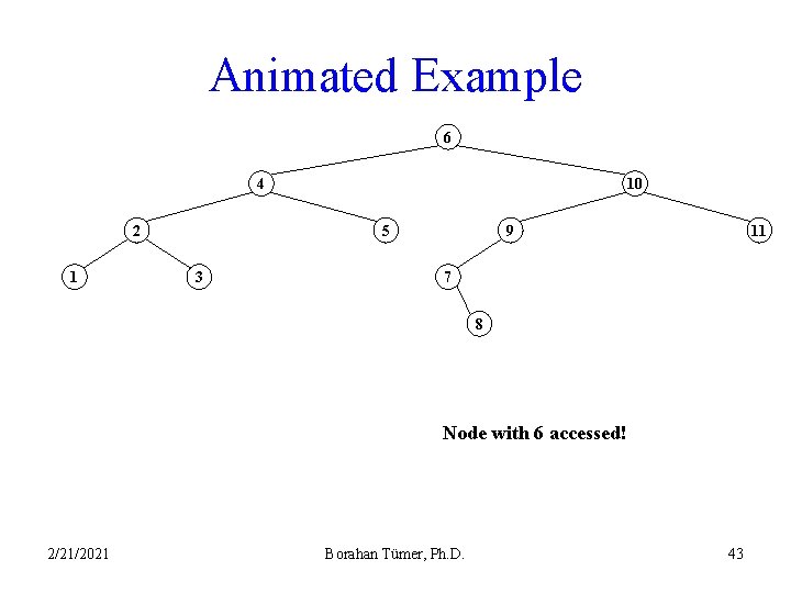
Animated Example 6 4 2 1 10 5 3 9 11 7 8 Node with 6 accessed! 2/21/2021 Borahan Tümer, Ph. D. 43

B-Trees 2/21/2021 Borahan Tümer, Ph. D. 44

Motivation for B-Trees • Two technologies for providing memory capacity in a computer system – Primary (main) memory (silicon chips) – Secondary storage (magnetic disks) • Primary memory – 5 orders of magnitude (i. e. , about 105 times) faster, – 2 orders of magnitude (about 100 times) more expensive, and – by at least 2 orders of magnitude less in size than secondary storage due to mechanical operations involved in magnetic disks. 2/21/2021 Borahan Tümer, Ph. D. 45

Motivation for B-Trees • During one disk read or disk write (4 -8. 5 msec for 7200 RPM disks), MM can be accessed about 105 times (100 nanosec per access). • To reimburse (compensate) for this time, at each disks access, not a single item, but one or more equal-sized pages of items (each page 211 -214 bytes) are accessed. • We need some data structure to store these equal sized pages in MM. • B-Trees, with their equal-sized leaves (as big as a page), are suitable data structures for storing and performing regular operations on paged data. 2/21/2021 Borahan Tümer, Ph. D. 46

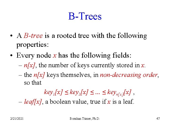
B-Trees • A B-tree is a rooted tree with the following properties: • Every node x has the following fields: – n[x], the number of keys currently stored in x. – the n[x] keys themselves, in non-decreasing order, so that key 1[x] ≤ key 2[x] ≤. . . ≤ keyn[x][x] , – leaf[x], a boolean value, true if x is a leaf. 2/21/2021 Borahan Tümer, Ph. D. 47

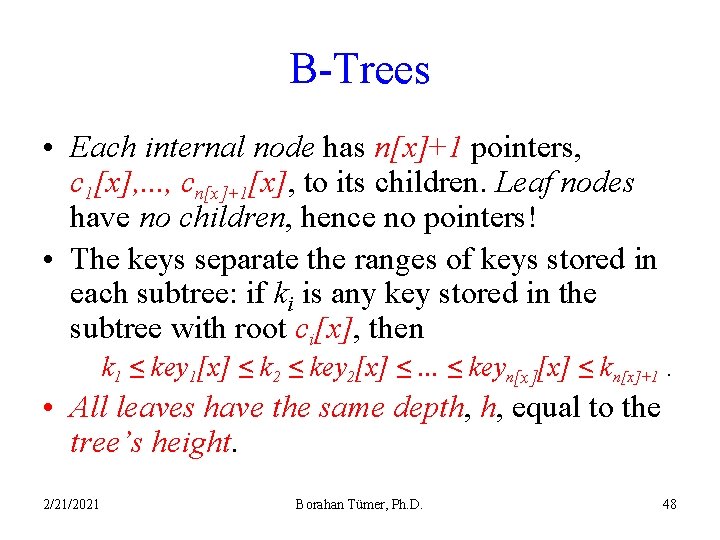
B-Trees • Each internal node has n[x]+1 pointers, c 1[x], . . . , cn[x]+1[x], to its children. Leaf nodes have no children, hence no pointers! • The keys separate the ranges of keys stored in each subtree: if ki is any key stored in the subtree with root ci[x], then k 1 ≤ key 1[x] ≤ k 2 ≤ key 2[x] ≤. . . ≤ keyn[x][x] ≤ kn[x]+1. • All leaves have the same depth, h, equal to the tree’s height. 2/21/2021 Borahan Tümer, Ph. D. 48

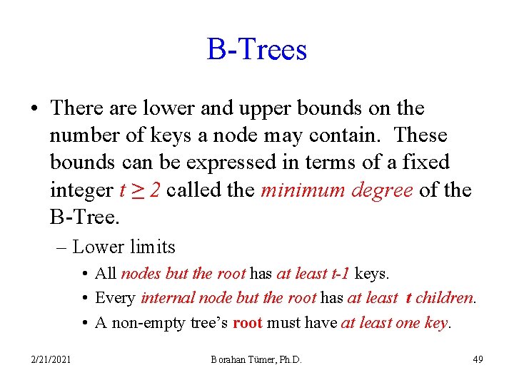
B-Trees • There are lower and upper bounds on the number of keys a node may contain. These bounds can be expressed in terms of a fixed integer t ≥ 2 called the minimum degree of the B-Tree. – Lower limits • All nodes but the root has at least t-1 keys. • Every internal node but the root has at least t children. • A non-empty tree’s root must have at least one key. 2/21/2021 Borahan Tümer, Ph. D. 49

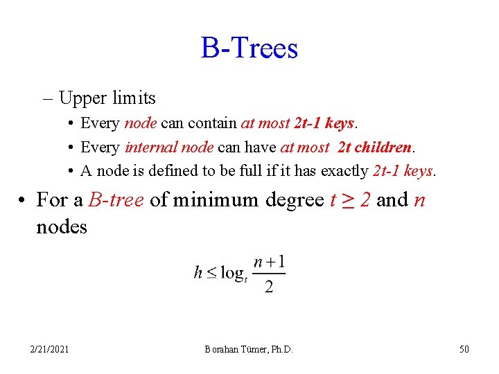
B-Trees – Upper limits • Every node can contain at most 2 t-1 keys. • Every internal node can have at most 2 t children. • A node is defined to be full if it has exactly 2 t-1 keys. • For a B-tree of minimum degree t ≥ 2 and n nodes 2/21/2021 Borahan Tümer, Ph. D. 50

Basic Operations on B-Trees • B-tree search • B-tree insert • B-tree removal 2/21/2021 Borahan Tümer, Ph. D. 51

Disk Operations in B-Tree operations • Suppose x is a pointer to an object. • It is accessible if it is in the main memory. • If it is on the disk, it needs to be transferred to the main memory to be accessible. This is done by DISK_READ(x). • To save any changes made to any field(s) of the object pointed to by x, a DISK_WRITE(x) operation is performed. 2/21/2021 Borahan Tümer, Ph. D. 52

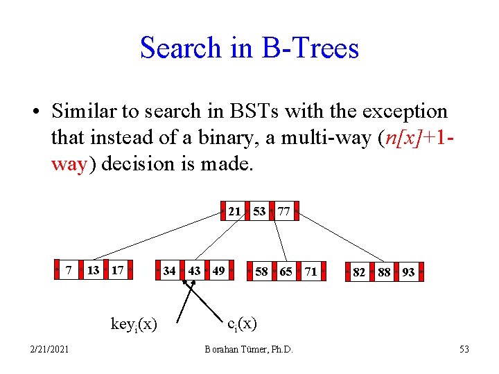
Search in B-Trees • Similar to search in BSTs with the exception that instead of a binary, a multi-way (n[x]+1 way) decision is made. 21 53 77 7 13 17 keyi(x) 2/21/2021 34 43 49 58 65 71 82 88 93 ci(x) Borahan Tümer, Ph. D. 53

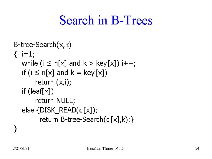
Search in B-Trees B-tree-Search(x, k) { i=1; while (i ≤ n[x] and k > keyi[x]) i++; if (i ≤ n[x] and k = keyi[x]) return (x, i); if (leaf[x]) return NULL; else {DISK_READ(ci[x]); return B-tree-Search(ci[x], k); } } 2/21/2021 Borahan Tümer, Ph. D. 54

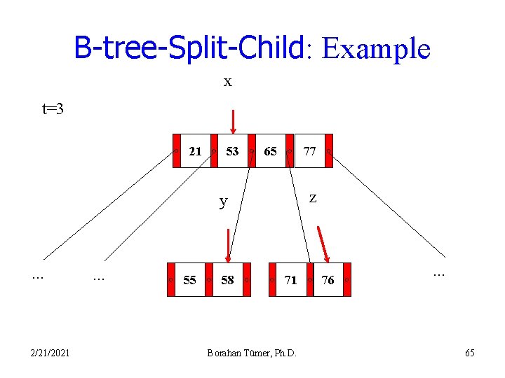
Insertion in B-Trees • Insertion into a B-tree is more complicated than that into a BST, since the creation of a new node to place the new key may violate the B-tree property of the tree. • Instead, the key is put into a leaf node x if it is not full. • If full, a split is applied, which splits a full node (with 2 t-1 keys) at its median key, keyt[x], into two nodes with t-1 keys each. • keyt[x] moves up into the parent of x and identifies the split point of the two new trees. 2/21/2021 Borahan Tümer, Ph. D. 55

Insertion in B-Trees • A single-pass insertion starts at the root traversing down to the leaf into which the key is to be inserted. • On the path down, all full nodes are split including a full leaf that also guarantees a parent with an available position for the median key of a full node to be placed. 2/21/2021 Borahan Tümer, Ph. D. 56

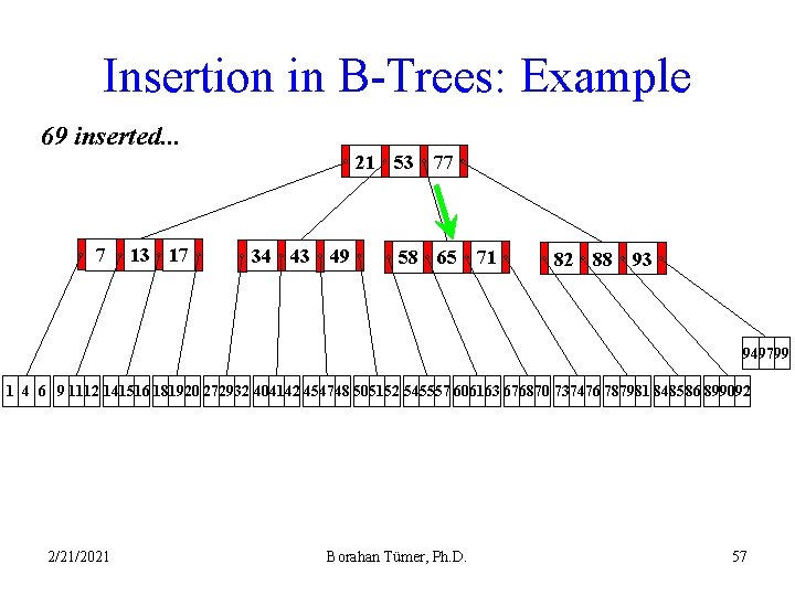
Insertion in B-Trees: Example 69 inserted. . . 21 53 77 7 13 17 34 43 49 58 65 71 82 88 93 949799 1 4 6 9 1112 141516 181920 272932 404142 454748 505152 545557 606163 676870 737476 787981 848586 899092 2/21/2021 Borahan Tümer, Ph. D. 57

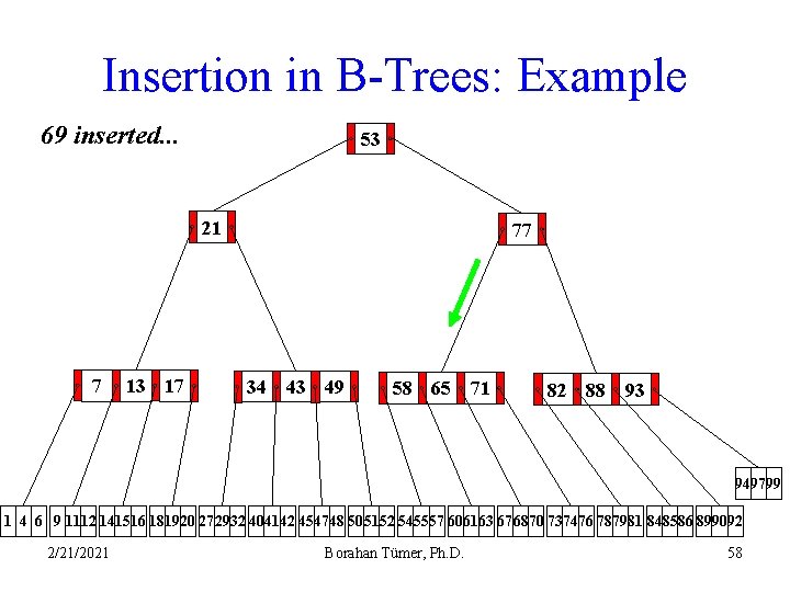
Insertion in B-Trees: Example 69 inserted. . . 53 21 7 13 17 77 34 43 49 58 65 71 82 88 93 949799 1 4 6 9 1112 141516 181920 272932 404142 454748 505152 545557 606163 676870 737476 787981 848586 899092 2/21/2021 Borahan Tümer, Ph. D. 58

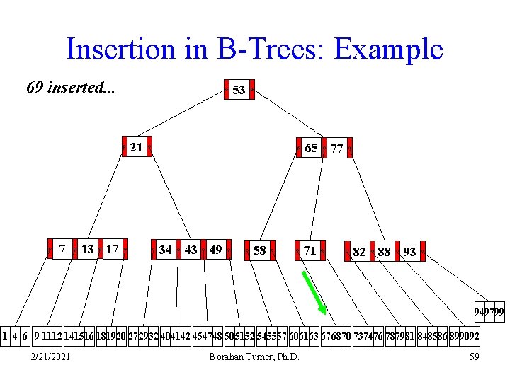
Insertion in B-Trees: Example 69 inserted. . . 53 21 7 13 17 65 34 43 49 58 71 77 82 88 93 949799 1 4 6 9 1112 141516 181920 272932 404142 454748 505152 545557 606163 676870 737476 787981 848586 899092 2/21/2021 Borahan Tümer, Ph. D. 59

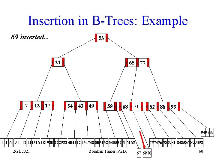
Insertion in B-Trees: Example 69 inserted. . . 53 21 7 13 17 65 34 43 49 58 68 77 71 82 88 93 949799 1 4 6 9 1112 141516 181920 272932 404142 454748 505152 545557 606163 2/21/2021 Borahan Tümer, Ph. D. 737476 787981 848586 899092 67 6970 60

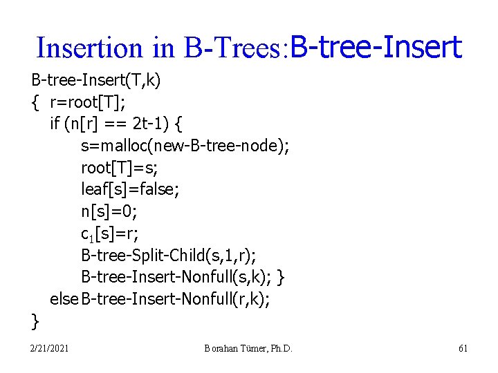
Insertion in B-Trees: B-tree-Insert(T, k) { r=root[T]; if (n[r] == 2 t-1) { s=malloc(new-B-tree-node); root[T]=s; leaf[s]=false; n[s]=0; c 1[s]=r; B-tree-Split-Child(s, 1, r); B-tree-Insert-Nonfull(s, k); } else B-tree-Insert-Nonfull(r, k); } 2/21/2021 Borahan Tümer, Ph. D. 61

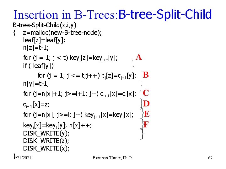
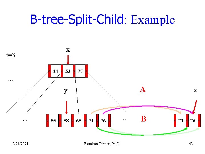
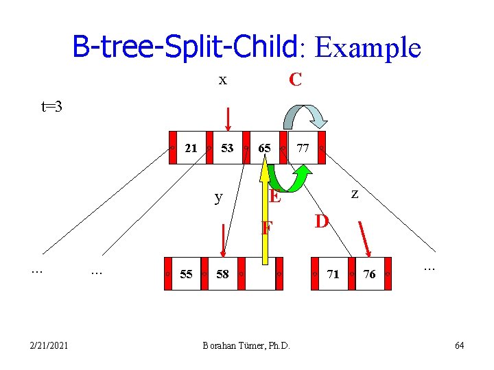
Insertion in B-Trees: B-tree-Split-Child(x, i, y) { z=malloc(new-B-tree-node); leaf[z]=leaf[y]; n[z]=t-1; for (j = 1; j < t) keyj[z]=keyj+t[y]; if (!leaf[y]) A for (j = 1; j <= t; j++) cj[z]=cj+t[y]; n[y]=t-1; B for (j=n[x]+1; j>=i+1; j--) cj+1[x]=cj[x]; C D E F ci+1[x]=z; for (j=n[x]; j>=i; j--) keyj+1[x]=keyj[x]; keyi[x]=keyt[y]; n[x]++; DISK_WRITE(y); DISK_WRITE(z); DISK_WRITE(x); }2/21/2021 Borahan Tümer, Ph. D. 62

B-tree-Split-Child: Example x t=3 21 53 77 . . . A y . . . 2/21/2021 55 58 65 71 76 Borahan Tümer, Ph. D. . B z 71 76 63

B-tree-Split-Child: Example C x t=3 21 53 y 65 2/21/2021 . . . 55 z E F . . . 77 58 Borahan Tümer, Ph. D. D 71 76 . . . 64

B-tree-Split-Child: Example x t=3 21 53 65 77 z y . . . 2/21/2021 . . . 55 58 71 Borahan Tümer, Ph. D. 76 . . . 65

Insertion in B-Trees: B-tree-Insert. Nonfull B-tree-Insert-Nonfull(x, k) { i=n[x]; if (leaf[x]) while (i≥ 1 and k < keyi[x]) {keyi+1[x]=keyi[x]; ; i--; } keyi+1[x]=k; n[x]++; DISK_WRITE(x); else { while (i≥ 1 and k < keyi[x]) i--; i++; DISK_READ(ci[x]); if (n[ci[x]]==2 t-1) { B-tree-Split-Child(x, i, ci[x]); if (k > keyi[x]) i++; } B-tree-Insert-Nonfull(ci[x], k); } } 2/21/2021 Borahan Tümer, Ph. D. if x is a leaf then place key in x; write x on disk; else find the node (root of subtree) key goes to; read node from disk; if node full split node at key’s position; recursive call with node split and key; 66

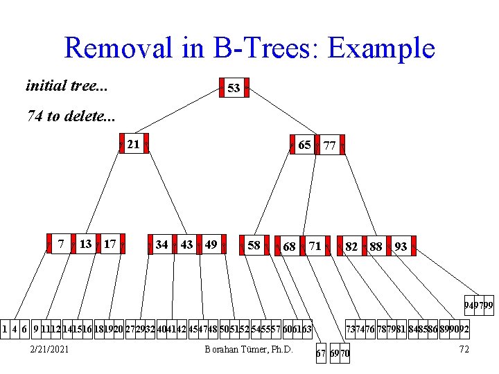
Removing a key from a B-Tree • Removal in B-trees is different than insertion only in that a key may be removed from any node, not just from a leaf. • As the insertion algorithm splits any full node down the path to the leaf to which the key is to be inserted, a recursive removal algorithm may be written to ensure that for any call to removal on a node x, the number of keys in x is at least the minimum degree t. 2/21/2021 Borahan Tümer, Ph. D. 67

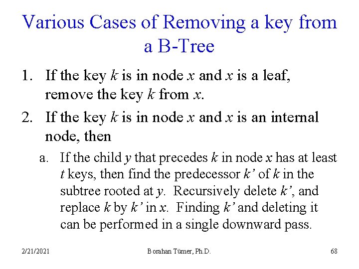
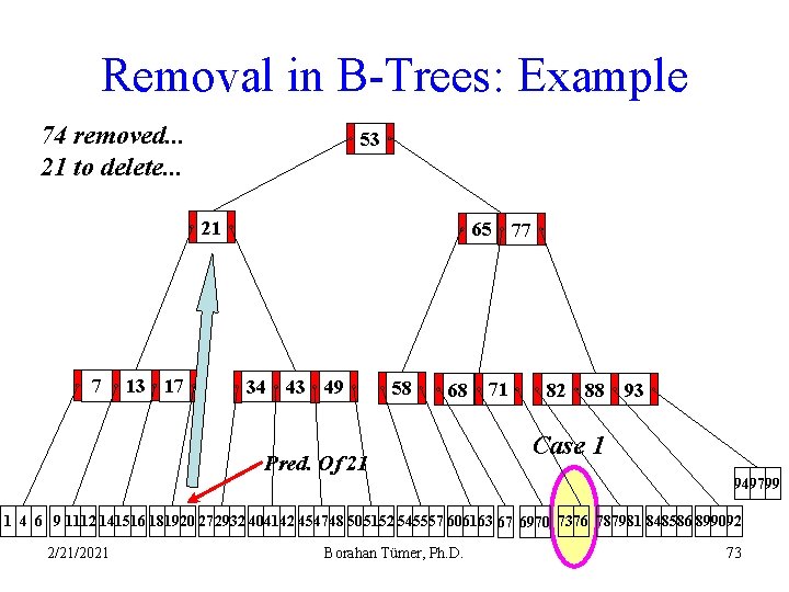
Various Cases of Removing a key from a B-Tree 1. If the key k is in node x and x is a leaf, remove the key k from x. 2. If the key k is in node x and x is an internal node, then a. If the child y that precedes k in node x has at least t keys, then find the predecessor k’ of k in the subtree rooted at y. Recursively delete k’, and replace k by k’ in x. Finding k’ and deleting it can be performed in a single downward pass. 2/21/2021 Borahan Tümer, Ph. D. 68

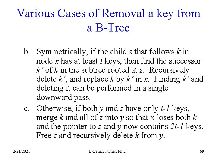
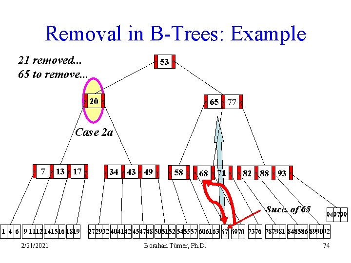
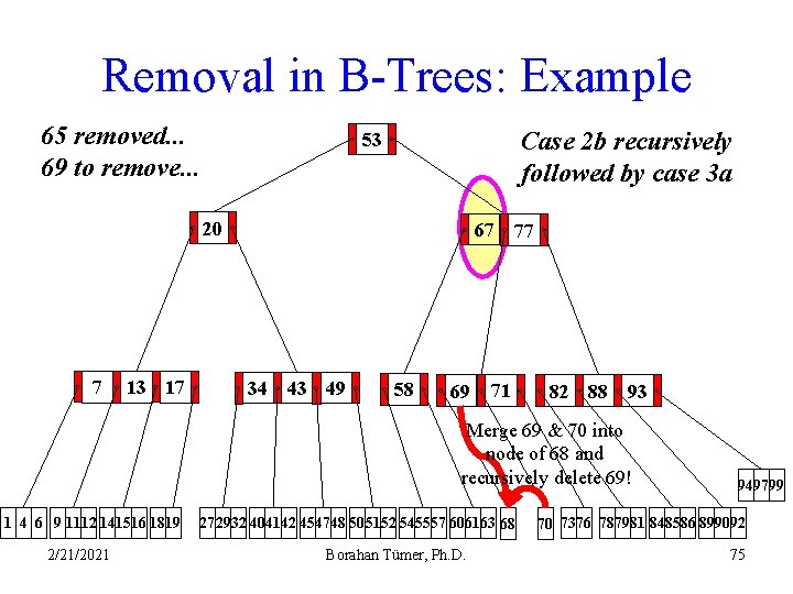
Various Cases of Removal a key from a B-Tree b. Symmetrically, if the child z that follows k in node x has at least t keys, then find the successor k’ of k in the subtree rooted at z. Recursively delete k’, and replace k by k’ in x. Finding k’ and deleting it can be performed in a single downward pass. c. Otherwise, if both y and z have only t-1 keys, merge k and all of z into y so that x loses both k and the pointer to z and y now contains 2 t-1 keys. Free z and recursively delete k from y. 2/21/2021 Borahan Tümer, Ph. D. 69

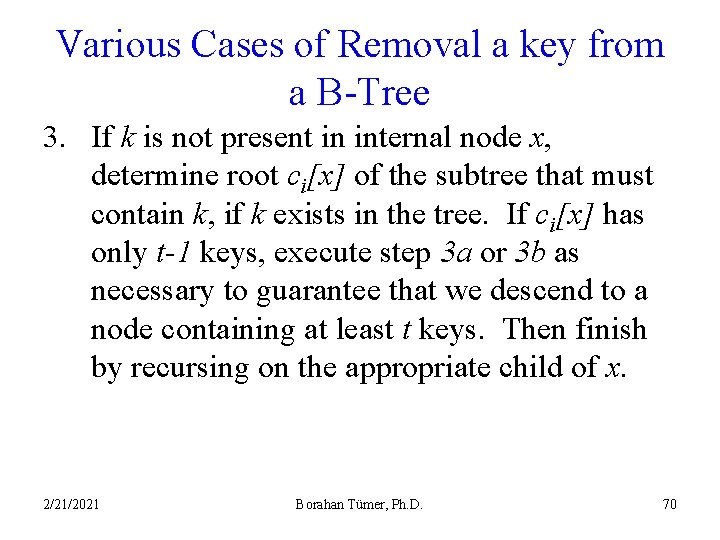
Various Cases of Removal a key from a B-Tree 3. If k is not present in internal node x, determine root ci[x] of the subtree that must contain k, if k exists in the tree. If ci[x] has only t-1 keys, execute step 3 a or 3 b as necessary to guarantee that we descend to a node containing at least t keys. Then finish by recursing on the appropriate child of x. 2/21/2021 Borahan Tümer, Ph. D. 70

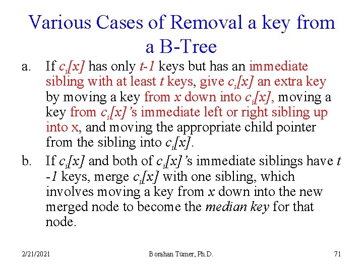
Various Cases of Removal a key from a B-Tree a. If ci[x] has only t-1 keys but has an immediate sibling with at least t keys, give ci[x] an extra key by moving a key from x down into ci[x], moving a key from ci[x]’s immediate left or right sibling up into x, and moving the appropriate child pointer from the sibling into ci[x]. b. If ci[x] and both of ci[x]’s immediate siblings have t -1 keys, merge ci[x] with one sibling, which involves moving a key from x down into the new merged node to become the median key for that node. 2/21/2021 Borahan Tümer, Ph. D. 71

Removal in B-Trees: Example initial tree. . . 53 74 to delete. . . 21 7 13 17 65 34 43 49 58 68 77 71 82 88 93 949799 1 4 6 9 1112 141516 181920 272932 404142 454748 505152 545557 606163 2/21/2021 Borahan Tümer, Ph. D. 737476 787981 848586 899092 67 6970 72

Removal in B-Trees: Example 74 removed. . . 21 to delete. . . 53 21 7 13 17 65 34 43 49 58 68 Pred. Of 21 71 77 82 88 93 Case 1 949799 1 4 6 9 1112 141516 181920 272932 404142 454748 505152 545557 606163 67 6970 7376 787981 848586 899092 2/21/2021 Borahan Tümer, Ph. D. 73

Removal in B-Trees: Example 21 removed. . . 65 to remove. . . 53 20 65 77 Case 2 a 7 13 17 34 43 49 58 68 71 82 88 93 Succ. of 65 1 4 6 9 1112 141516 1819 2/21/2021 949799 272932 404142 454748 505152 545557 606163 67 6970 7376 787981 848586 899092 Borahan Tümer, Ph. D. 74

Removal in B-Trees: Example 65 removed. . . 69 to remove. . . Case 2 b recursively followed by case 3 a 53 20 7 13 17 67 34 43 49 58 69 77 71 82 88 93 Merge 69 & 70 into node of 68 and recursively delete 69! 1 4 6 9 1112 141516 1819 2/21/2021 272932 404142 454748 505152 545557 606163 68 Borahan Tümer, Ph. D. 949799 70 7376 787981 848586 899092 75

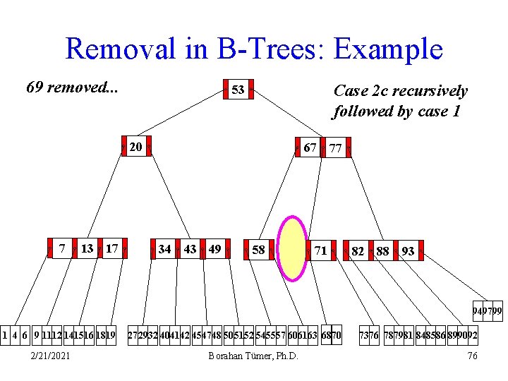
Removal in B-Trees: Example 69 removed. . . Case 2 c recursively followed by case 1 53 20 7 13 17 67 34 43 49 58 77 71 82 88 93 949799 1 4 6 9 1112 141516 1819 2/21/2021 272932 404142 454748 505152 545557 606163 6870 Borahan Tümer, Ph. D. 7376 787981 848586 899092 76