Design and Analysis of MultiFactored Experiments Twolevel Factorial

Design and Analysis of Multi-Factored Experiments Two-level Factorial Designs L. M. Lye DOE Course 1

The 2 k Factorial Design • Special case of the general factorial design; k factors, all at two levels • The two levels are usually called low and high (they could be either quantitative or qualitative) • Very widely used in industrial experimentation • Form a basic “building block” for other very useful experimental designs (DNA) • Special (short-cut) methods for analysis • We will make use of Design-Expert for analysis L. M. Lye DOE Course 2

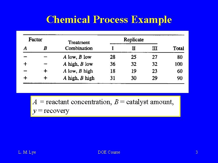
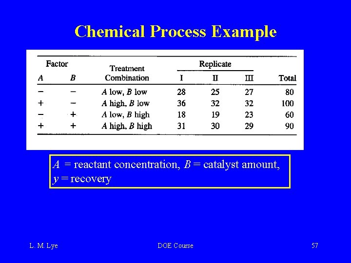
Chemical Process Example A = reactant concentration, B = catalyst amount, y = recovery L. M. Lye DOE Course 3

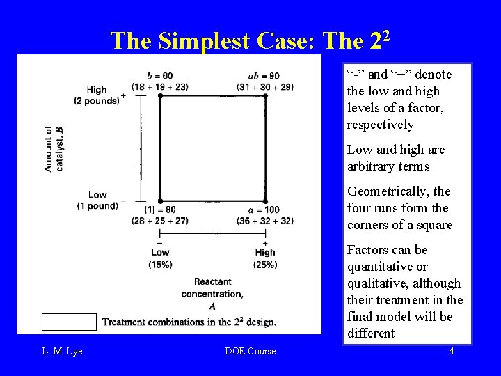
The Simplest Case: The 22 “-” and “+” denote the low and high levels of a factor, respectively Low and high are arbitrary terms Geometrically, the four runs form the corners of a square Factors can be quantitative or qualitative, although their treatment in the final model will be different L. M. Lye DOE Course 4

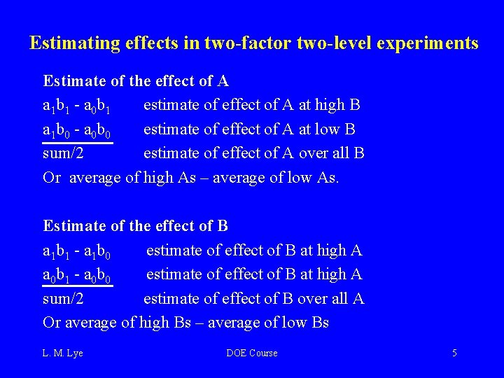
Estimating effects in two-factor two-level experiments Estimate of the effect of A a 1 b 1 - a 0 b 1 estimate of effect of A at high B a 1 b 0 - a 0 b 0 estimate of effect of A at low B sum/2 estimate of effect of A over all B Or average of high As – average of low As. Estimate of the effect of B a 1 b 1 - a 1 b 0 estimate of effect of B at high A a 0 b 1 - a 0 b 0 estimate of effect of B at high A sum/2 estimate of effect of B over all A Or average of high Bs – average of low Bs L. M. Lye DOE Course 5

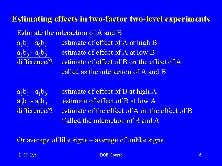
Estimating effects in two-factor two-level experiments Estimate the interaction of A and B a 1 b 1 - a 0 b 1 estimate of effect of A at high B a 1 b 0 - a 0 b 0 estimate of effect of A at low B difference/2 estimate of effect of B on the effect of A called as the interaction of A and B a 1 b 1 - a 1 b 0 a 0 b 1 - a 0 b 0 difference/2 estimate of effect of B at high A estimate of effect of B at low A estimate of the effect of A on the effect of B Called the interaction of B and A Or average of like signs – average of unlike signs L. M. Lye DOE Course 6

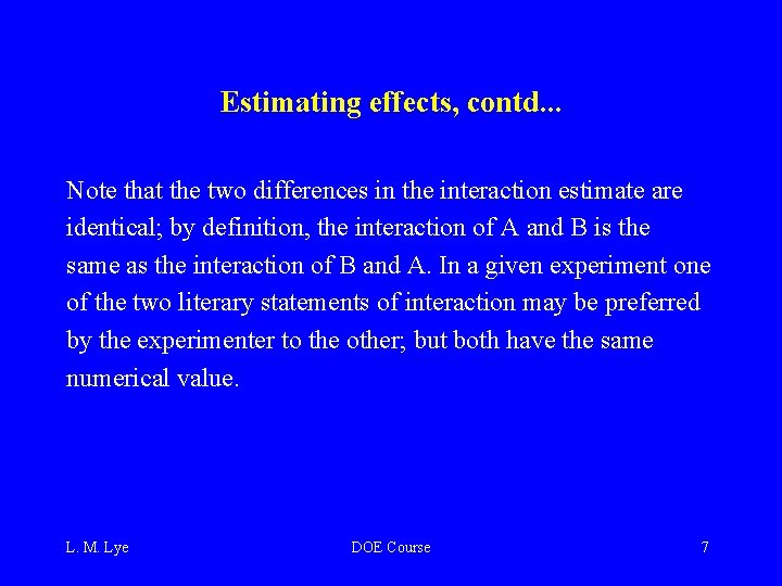
Estimating effects, contd. . . Note that the two differences in the interaction estimate are identical; by definition, the interaction of A and B is the same as the interaction of B and A. In a given experiment one of the two literary statements of interaction may be preferred by the experimenter to the other; but both have the same numerical value. L. M. Lye DOE Course 7

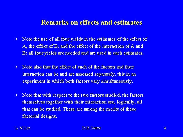
Remarks on effects and estimates • Note the use of all four yields in the estimates of the effect of A, the effect of B, and the effect of the interaction of A and B; all four yields are needed and are used in each estimates. • Note also that the effect of each of the factors and their interaction can be and are assessed separately, this in an experiment in which both factors vary simultaneously. • Note that with respect to the two factors studied, the factors themselves together with their interaction are, logically, all that can be studied. These are among the merits of these factorial designs. L. M. Lye DOE Course 8

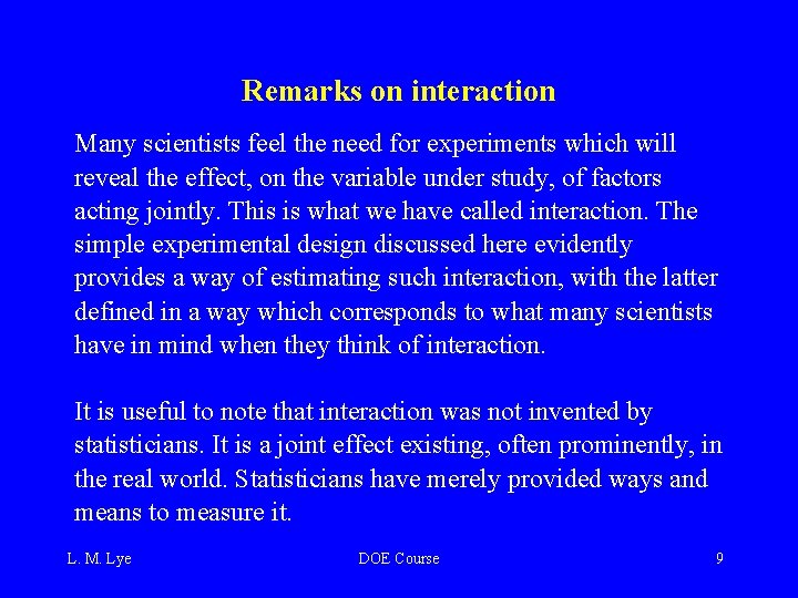
Remarks on interaction Many scientists feel the need for experiments which will reveal the effect, on the variable under study, of factors acting jointly. This is what we have called interaction. The simple experimental design discussed here evidently provides a way of estimating such interaction, with the latter defined in a way which corresponds to what many scientists have in mind when they think of interaction. It is useful to note that interaction was not invented by statisticians. It is a joint effect existing, often prominently, in the real world. Statisticians have merely provided ways and means to measure it. L. M. Lye DOE Course 9

Symbolism and language A is called a main effect. Our estimate of A is often simply written A. B is called a main effect. Our estimate of B is often simply written B. AB is called an interaction effect. Our estimate of AB is often simply written AB. So the same letter is used, generally without confusion, to describe the factor, to describe its effect, and to describe our estimate of its effect. Keep in mind that it is only for economy in writing that we sometimes speak of an effect rather than an estimate of the effect. We should always remember that all quantities formed from the yields are merely estimates. L. M. Lye DOE Course 10

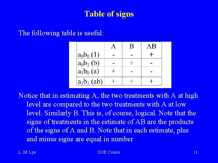
Table of signs The following table is useful: Notice that in estimating A, the two treatments with A at high level are compared to the two treatments with A at low level. Similarly B. This is, of course, logical. Note that the signs of treatments in the estimate of AB are the products of the signs of A and B. Note that in each estimate, plus and minus signs are equal in number L. M. Lye DOE Course 11

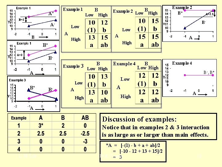
Example 1 A+ B Low High Example 2 Low B High Example 2 B+ A=2. 5 B=2 A- B- Low A B A High B+ A=3 BExample 3 A Example 3 15 14 13 12 Y 11 10 9 Low B+ B- A High -2 -1 A 0 B Low High Example 4 B- , B+ Low A High A 1 Discussion of examples: Notice that in examples 2 & 3 interaction is as large as or larger than main effects. L. M. Lye *A = [-(1) - b + ab]/2 = [-10 - 12 + 13 + 15]/2 DOE Course = 3 12

• Change of scale, by multiplying each yield by a constant, multiplies each estimate by the constant but does not affect the relationship of estimates to each other. • Addition of a constant to each yield does not affect the estimates. • The numerical magnitude of estimates is not important here; it is their relationship to each other. L. M. Lye DOE Course 13

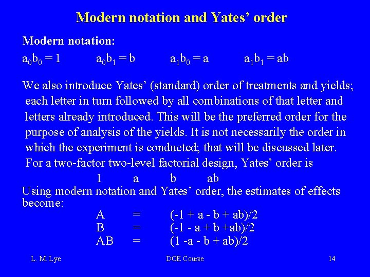
Modern notation and Yates’ order Modern notation: a 0 b 0 = 1 a 0 b 1 = b a 1 b 0 = a a 1 b 1 = ab We also introduce Yates’ (standard) order of treatments and yields; each letter in turn followed by all combinations of that letter and letters already introduced. This will be the preferred order for the purpose of analysis of the yields. It is not necessarily the order in which the experiment is conducted; that will be discussed later. For a two-factor two-level factorial design, Yates’ order is 1 a b ab Using modern notation and Yates’ order, the estimates of effects become: A = (-1 + a - b + ab)/2 B = (-1 - a + b +ab)/2 AB = (1 -a - b + ab)/2 L. M. Lye DOE Course 14

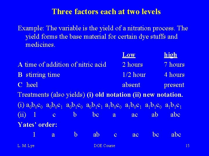
Three factors each at two levels Example: The variable is the yield of a nitration process. The yield forms the base material for certain dye stuffs and medicines. Low high A time of addition of nitric acid 2 hours 7 hours B stirring time 1/2 hour 4 hours C heel absent present Treatments (also yields) (i) old notation (ii) new notation. (i) a 0 b 0 c 0 a 0 b 0 c 1 a 0 b 1 c 0 a 0 b 1 c 1 a 1 b 0 c 0 a 1 b 0 c 1 a 1 b 1 c 0 a 1 b 1 c 1 (ii) 1 c b bc a ac ab abc Yates’ order: 1 a b ab c ac bc abc L. M. Lye DOE Course 15

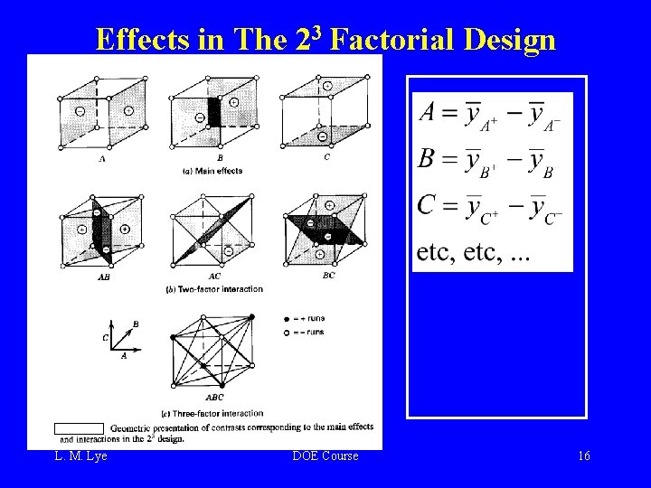
Effects in The 23 Factorial Design L. M. Lye DOE Course 16

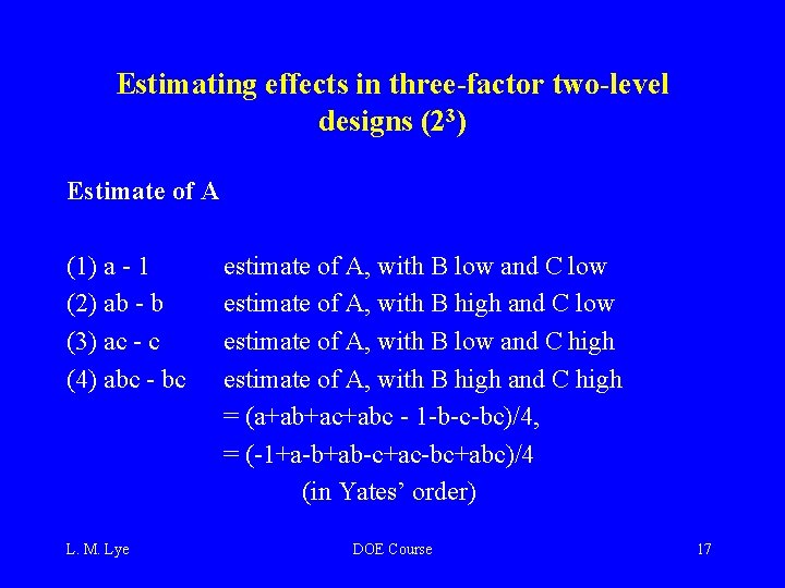
Estimating effects in three-factor two-level designs (23) Estimate of A (1) a - 1 (2) ab - b (3) ac - c (4) abc - bc L. M. Lye estimate of A, with B low and C low estimate of A, with B high and C low estimate of A, with B low and C high estimate of A, with B high and C high = (a+ab+ac+abc - 1 -b-c-bc)/4, = (-1+a-b+ab-c+ac-bc+abc)/4 (in Yates’ order) DOE Course 17

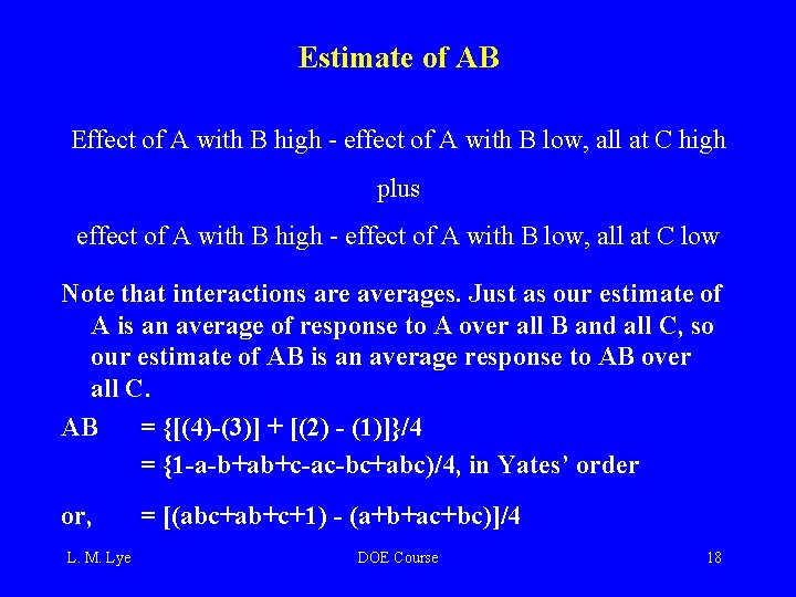
Estimate of AB Effect of A with B high - effect of A with B low, all at C high plus effect of A with B high - effect of A with B low, all at C low Note that interactions are averages. Just as our estimate of A is an average of response to A over all B and all C, so our estimate of AB is an average response to AB over all C. AB = {[(4)-(3)] + [(2) - (1)]}/4 = {1 -a-b+ab+c-ac-bc+abc)/4, in Yates’ order or, L. M. Lye = [(abc+ab+c+1) - (a+b+ac+bc)]/4 DOE Course 18

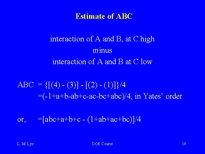
Estimate of ABC interaction of A and B, at C high minus interaction of A and B at C low ABC = {[(4) - (3)] - [(2) - (1)]}/4 =(-1+a+b-ab+c-ac-bc+abc)/4, in Yates’ order or, L. M. Lye =[abc+a+b+c - (1+ab+ac+bc)]/4 DOE Course 19

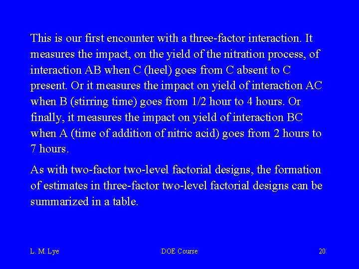
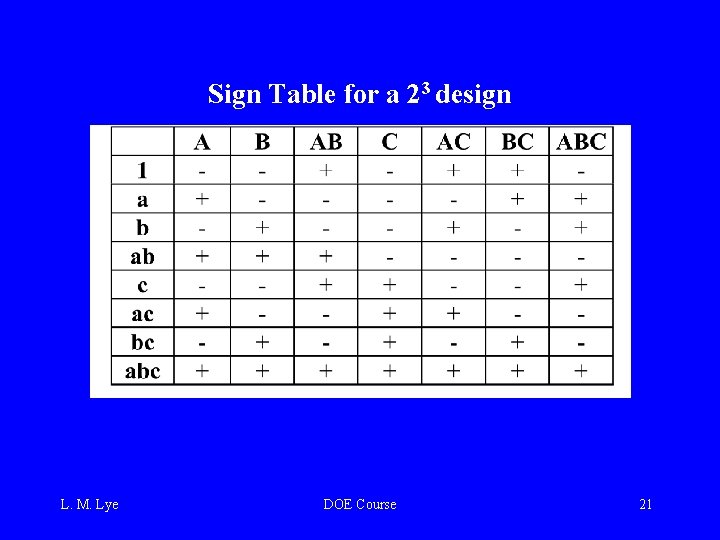
This is our first encounter with a three-factor interaction. It measures the impact, on the yield of the nitration process, of interaction AB when C (heel) goes from C absent to C present. Or it measures the impact on yield of interaction AC when B (stirring time) goes from 1/2 hour to 4 hours. Or finally, it measures the impact on yield of interaction BC when A (time of addition of nitric acid) goes from 2 hours to 7 hours. As with two-factor two-level factorial designs, the formation of estimates in three-factor two-level factorial designs can be summarized in a table. L. M. Lye DOE Course 20

Sign Table for a 23 design L. M. Lye DOE Course 21

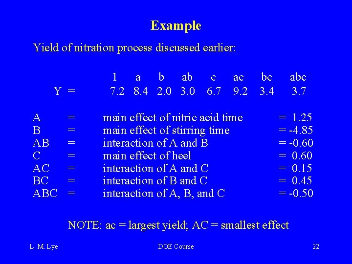
Example Yield of nitration process discussed earlier: Y = A B AB C AC BC ABC = = = = 1 a b ab 7. 2 8. 4 2. 0 3. 0 c 6. 7 ac 9. 2 main effect of nitric acid time main effect of stirring time interaction of A and B main effect of heel interaction of A and C interaction of B and C interaction of A, B, and C bc 3. 4 abc 3. 7 = 1. 25 = -4. 85 = -0. 60 = 0. 15 = 0. 45 = -0. 50 NOTE: ac = largest yield; AC = smallest effect L. M. Lye DOE Course 22

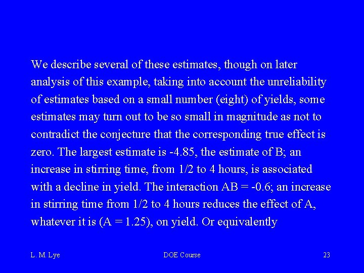
We describe several of these estimates, though on later analysis of this example, taking into account the unreliability of estimates based on a small number (eight) of yields, some estimates may turn out to be so small in magnitude as not to contradict the conjecture that the corresponding true effect is zero. The largest estimate is -4. 85, the estimate of B; an increase in stirring time, from 1/2 to 4 hours, is associated with a decline in yield. The interaction AB = -0. 6; an increase in stirring time from 1/2 to 4 hours reduces the effect of A, whatever it is (A = 1. 25), on yield. Or equivalently L. M. Lye DOE Course 23

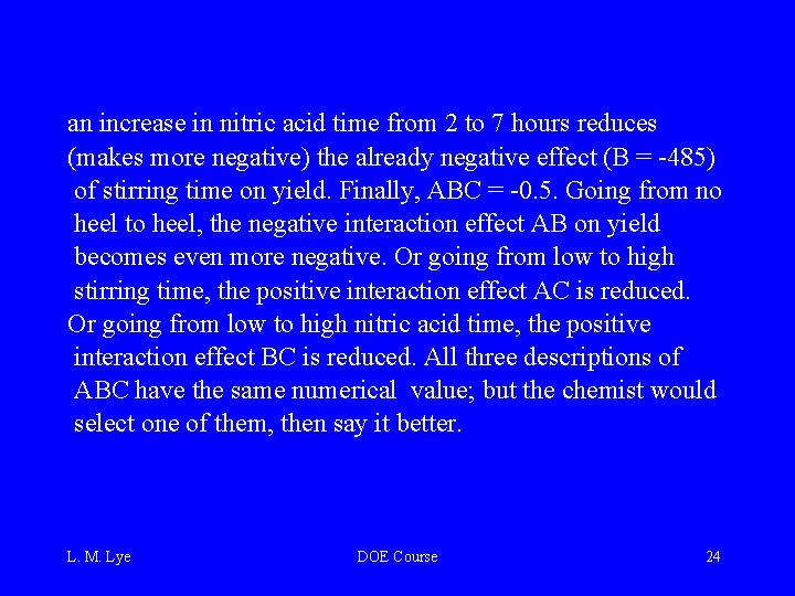
an increase in nitric acid time from 2 to 7 hours reduces (makes more negative) the already negative effect (B = -485) of stirring time on yield. Finally, ABC = -0. 5. Going from no heel to heel, the negative interaction effect AB on yield becomes even more negative. Or going from low to high stirring time, the positive interaction effect AC is reduced. Or going from low to high nitric acid time, the positive interaction effect BC is reduced. All three descriptions of ABC have the same numerical value; but the chemist would select one of them, then say it better. L. M. Lye DOE Course 24

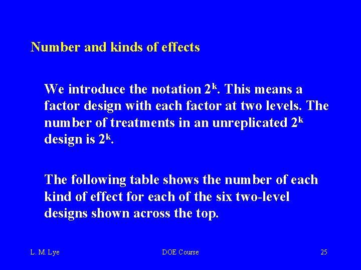
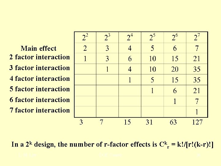
Number and kinds of effects We introduce the notation 2 k. This means a factor design with each factor at two levels. The number of treatments in an unreplicated 2 k design is 2 k. The following table shows the number of each kind of effect for each of the six two-level designs shown across the top. L. M. Lye DOE Course 25

Main effect 2 factor interaction 3 factor interaction 4 factor interaction 5 factor interaction 6 factor interaction 7 factor interaction 3 7 15 31 63 127 In a 2 k design, the number of r-factor effects is Ckr = k!/[r!(k-r)!] L. M. Lye DOE Course 26

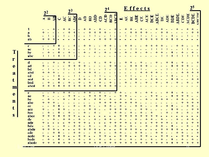
Notice that the total number of effects estimated in any design is always one less than the number of treatments In a 22 design, there are 22=4 treatments; we estimate 22 -1 = 3 effects. In a 23 design, there are 23=8 treatments; we estimate 231 = 7 effects One need not repeat the earlier logic to determine the forms of estimates in 2 k designs for higher values of k. A table going up to 25 follows. L. M. Lye DOE Course 27

22 23 24 25 Effects T r e a t m e n t s L. M. Lye DOE Course 28

Yates’ Forward Algorithm (1) 1. Applied to Complete Factorials (Yates, 1937) A systematic method of calculating estimates of effects. For complete factorials first arrange the yields in Yates’ (standard) order. Addition, then subtraction of adjacent yields. The addition and subtraction operations are repeated until 2 k terms appear in each line: for a 2 k there will be k columns of calculations L. M. Lye DOE Course 29

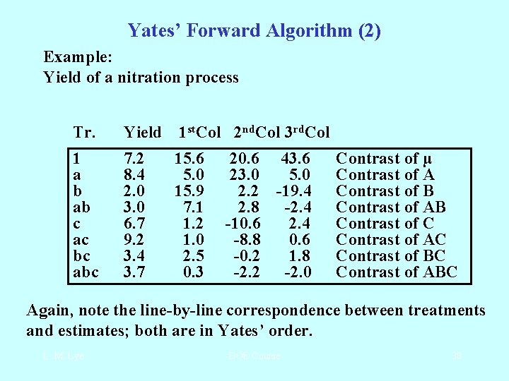
Yates’ Forward Algorithm (2) Example: Yield of a nitration process Tr. Yield 1 st. Col 2 nd. Col 3 rd. Col 1 a b ab c ac bc abc 7. 2 8. 4 2. 0 3. 0 6. 7 9. 2 3. 4 3. 7 15. 6 5. 0 15. 9 7. 1 1. 2 1. 0 2. 5 0. 3 20. 6 43. 6 23. 0 5. 0 2. 2 -19. 4 2. 8 -2. 4 -10. 6 2. 4 -8. 8 0. 6 -0. 2 1. 8 -2. 2 -2. 0 Contrast of µ Contrast of A Contrast of B Contrast of AB Contrast of C Contrast of AC Contrast of BC Contrast of ABC Again, note the line-by-line correspondence between treatments and estimates; both are in Yates’ order. L. M. Lye DOE Course 30

Main effects in the face of large interactions Several writers have cautioned against making statements about main effects when the corresponding interactions are large; interactions describe the dependence of the impact of one factor on the level of another; in the presence of large interaction, main effects may not be meaningful. L. M. Lye DOE Course 31

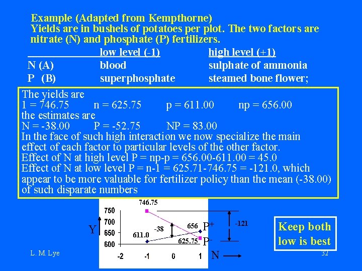
Example (Adapted from Kempthorne) Yields are in bushels of potatoes per plot. The two factors are nitrate (N) and phosphate (P) fertilizers. low level (-1) high level (+1) N (A) blood sulphate of ammonia P (B) superphosphate steamed bone flower; The yields are 1 = 746. 75 n = 625. 75 p = 611. 00 np = 656. 00 the estimates are N = -38. 00 P = -52. 75 NP = 83. 00 In the face of such high interaction we now specialize the main effect of each factor to particular levels of the other factor. Effect of N at high level P = np-p = 656. 00 -611. 00 = 45. 0 Effect of N at low level P = n-1 = 625. 71 -746. 75 = -121. 0, which appear to be more valuable for fertilizer policy than the mean (-38. 00) of such disparate numbers 746. 75 Y L. M. Lye 611. 0 -38 656 625. 75 DOE Course P+ PN -121 Keep both low is best 32

Note that answers to these specialized questions are based on fewer than 2 k yields. In our numerical example, with interaction NP prominent, we have only two of the four yields in our estimate of N at each level of P. In general we accept high interactions wherever found and seek to explain them; in the process of explanation, main effects (and lower-order interactions) may have to be replaced in our interest by more meaningful specialized or conditional effects. L. M. Lye DOE Course 33

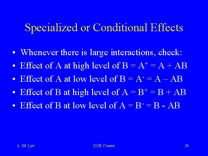
Specialized or Conditional Effects • • • Whenever there is large interactions, check: Effect of A at high level of B = A+ = A + AB Effect of A at low level of B = A- = A – AB Effect of B at high level of A = B+ = B + AB Effect of B at low level of A = B- = B - AB L. M. Lye DOE Course 34

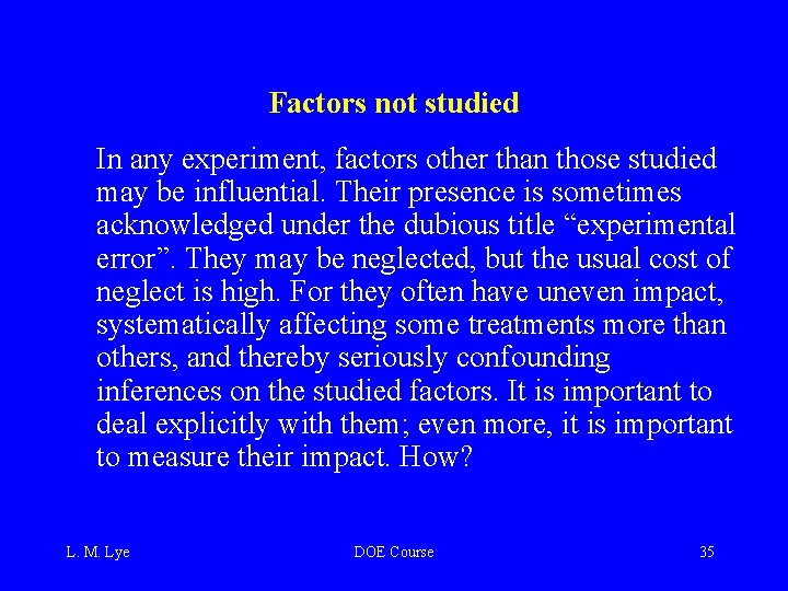
Factors not studied In any experiment, factors other than those studied may be influential. Their presence is sometimes acknowledged under the dubious title “experimental error”. They may be neglected, but the usual cost of neglect is high. For they often have uneven impact, systematically affecting some treatments more than others, and thereby seriously confounding inferences on the studied factors. It is important to deal explicitly with them; even more, it is important to measure their impact. How? L. M. Lye DOE Course 35

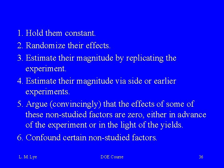
1. Hold them constant. 2. Randomize their effects. 3. Estimate their magnitude by replicating the experiment. 4. Estimate their magnitude via side or earlier experiments. 5. Argue (convincingly) that the effects of some of these non-studied factors are zero, either in advance of the experiment or in the light of the yields. 6. Confound certain non-studied factors. L. M. Lye DOE Course 36

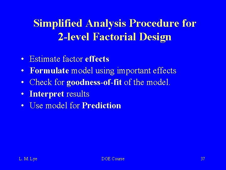
Simplified Analysis Procedure for 2 -level Factorial Design • • • Estimate factor effects Formulate model using important effects Check for goodness-of-fit of the model. Interpret results Use model for Prediction L. M. Lye DOE Course 37

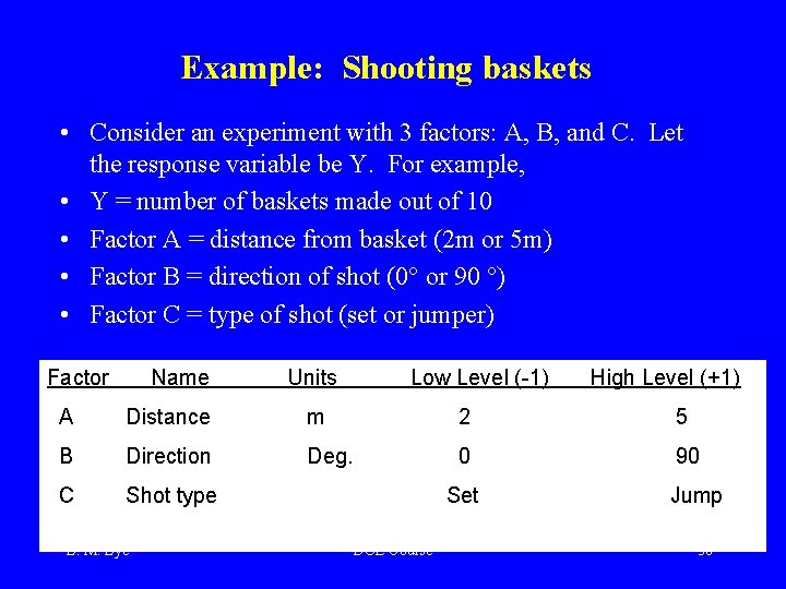
Example: Shooting baskets • Consider an experiment with 3 factors: A, B, and C. Let the response variable be Y. For example, • Y = number of baskets made out of 10 • Factor A = distance from basket (2 m or 5 m) • Factor B = direction of shot (0° or 90 °) • Factor C = type of shot (set or jumper) Factor Name Units Low Level (-1) High Level (+1) A Distance m 2 5 B Direction Deg. 0 90 C Shot type L. M. Lye Set DOE Course Jump 38

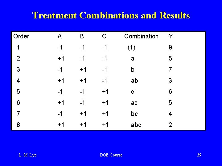
Treatment Combinations and Results Order A B C 1 -1 -1 -1 (1) 9 2 +1 -1 -1 a 5 3 -1 +1 -1 b 7 4 +1 +1 -1 ab 3 5 -1 -1 +1 c 6 6 +1 -1 +1 ac 5 7 -1 +1 +1 bc 4 8 +1 +1 +1 abc 2 L. M. Lye DOE Course Combination Y 39

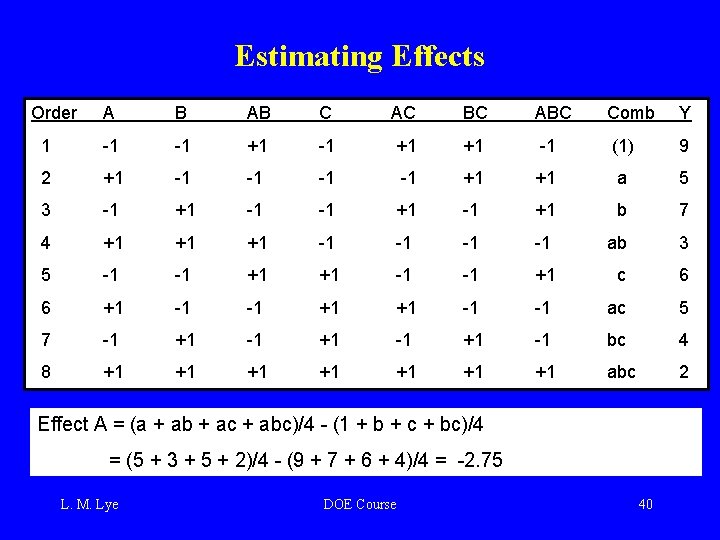
Estimating Effects Order A B AB C AC BC ABC Comb Y 1 -1 -1 +1 +1 -1 (1) 9 2 +1 -1 -1 +1 +1 a 5 3 -1 +1 b 7 4 +1 +1 +1 -1 -1 ab 3 5 -1 -1 +1 +1 -1 -1 +1 c 6 6 +1 -1 -1 +1 +1 -1 -1 ac 5 7 -1 +1 -1 bc 4 8 +1 +1 abc 2 Effect A = (a + ab + ac + abc)/4 - (1 + b + c + bc)/4 = (5 + 3 + 5 + 2)/4 - (9 + 7 + 6 + 4)/4 = -2. 75 L. M. Lye DOE Course 40

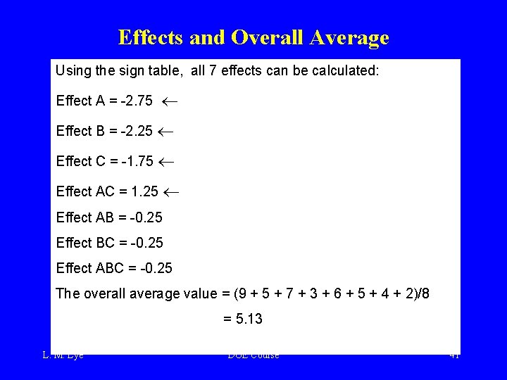
Effects and Overall Average Using the sign table, all 7 effects can be calculated: Effect A = -2. 75 Effect B = -2. 25 Effect C = -1. 75 Effect AC = 1. 25 Effect AB = -0. 25 Effect BC = -0. 25 Effect ABC = -0. 25 The overall average value = (9 + 5 + 7 + 3 + 6 + 5 + 4 + 2)/8 = 5. 13 L. M. Lye DOE Course 41

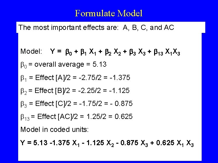
Formulate Model The most important effects are: A, B, C, and AC Model: Y = b 0 + b 1 X 1 + b 2 X 2 + b 3 X 3 + b 13 X 1 X 3 b 0 = overall average = 5. 13 b 1 = Effect [A]/2 = -2. 75/2 = -1. 375 b 2 = Effect [B]/2 = -2. 25/2 = -1. 125 b 3 = Effect [C]/2 = -1. 75/2 = - 0. 875 b 13 = Effect [AC]/2 = 1. 25/2 = 0. 625 Model in coded units: Y = 5. 13 -1. 375 X 1 - 1. 125 X 2 - 0. 875 X 3 + 0. 625 X 1 X 3 L. M. Lye DOE Course 42

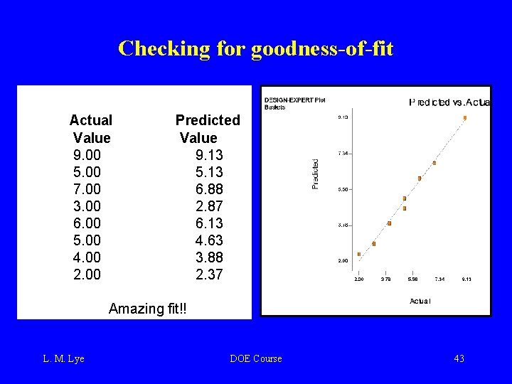
Checking for goodness-of-fit Actual Value 9. 00 5. 00 7. 00 3. 00 6. 00 5. 00 4. 00 2. 00 Predicted Value 9. 13 5. 13 6. 88 2. 87 6. 13 4. 63 3. 88 2. 37 Amazing fit!! L. M. Lye DOE Course 43

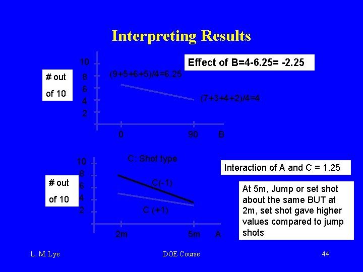
Interpreting Results 10 # out of 10 8 6 4 2 Effect of B=4 -6. 25= -2. 25 (9+5+6+5)/4=6. 25 (7+3+4+2)/4=4 0 10 8 # out 6 of 10 4 2 90 C: Shot type Interaction of A and C = 1. 25 C(-1) C (+1) 2 m L. M. Lye B 5 m DOE Course A At 5 m, Jump or set shot about the same BUT at 2 m, set shot gave higher values compared to jump shots 44

Design and Analysis of Multi-Factored Experiments Analysis of 2 k Experiments Statistical Details L. M. Lye DOE Course 45

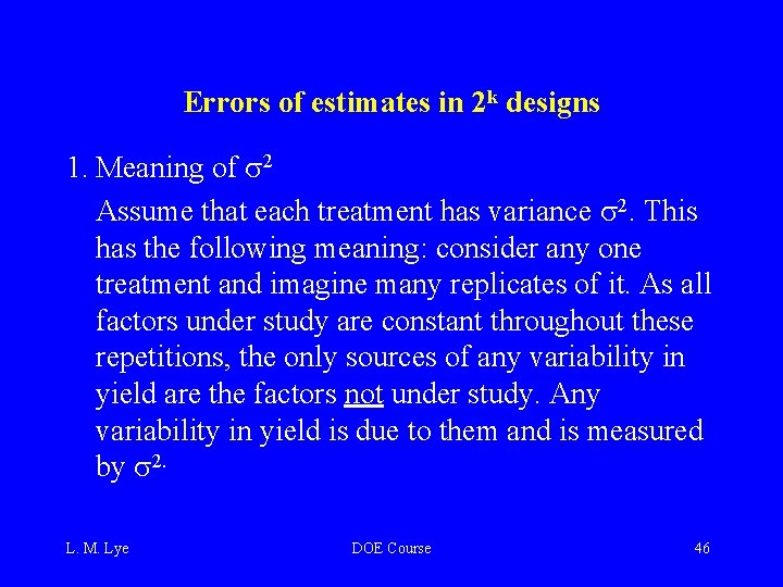
Errors of estimates in 2 k designs 1. Meaning of 2 Assume that each treatment has variance 2. This has the following meaning: consider any one treatment and imagine many replicates of it. As all factors under study are constant throughout these repetitions, the only sources of any variability in yield are the factors not under study. Any variability in yield is due to them and is measured by 2. L. M. Lye DOE Course 46

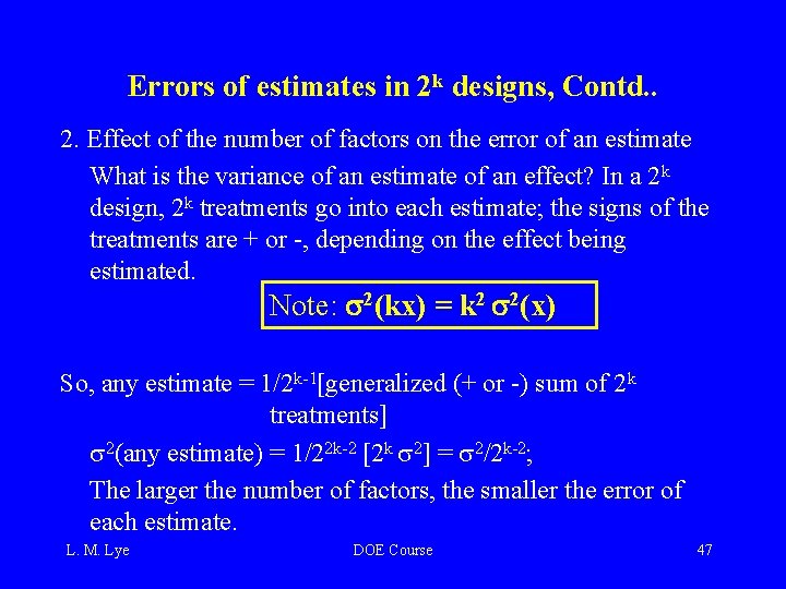
Errors of estimates in 2 k designs, Contd. . 2. Effect of the number of factors on the error of an estimate What is the variance of an estimate of an effect? In a 2 k design, 2 k treatments go into each estimate; the signs of the treatments are + or -, depending on the effect being estimated. Note: 2(kx) = k 2 2(x) So, any estimate = 1/2 k-1[generalized (+ or -) sum of 2 k treatments] 2(any estimate) = 1/22 k-2 [2 k 2] = 2/2 k-2; The larger the number of factors, the smaller the error of each estimate. L. M. Lye DOE Course 47

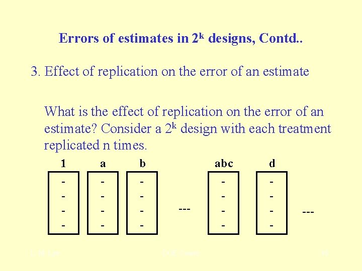
Errors of estimates in 2 k designs, Contd. . 3. Effect of replication on the error of an estimate What is the effect of replication on the error of an estimate? Consider a 2 k design with each treatment replicated n times. L. M. Lye 1 a b abc d - - --- DOE Course --- 48

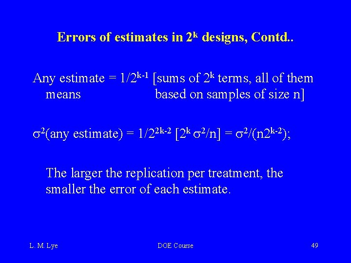
Errors of estimates in 2 k designs, Contd. . Any estimate = 1/2 k-1 [sums of 2 k terms, all of them means based on samples of size n] 2(any estimate) = 1/22 k-2 [2 k 2/n] = 2/(n 2 k-2); The larger the replication per treatment, the smaller the error of each estimate. L. M. Lye DOE Course 49

So, the error of an estimate depends on k (the number of factors studied) and n (the replication per factor). It also (obviously) depends on 2. The variance 2 can be reduced holding some of the non-studied factors constant. But, as has been noted, this gain is offset by reduced generality of any conclusions. L. M. Lye DOE Course 50

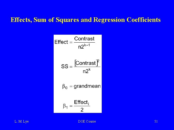
Effects, Sum of Squares and Regression Coefficients L. M. Lye DOE Course 51

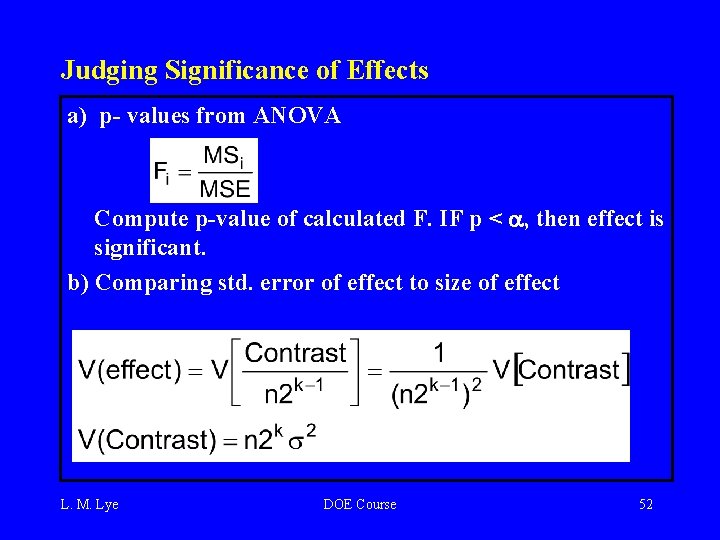
Judging Significance of Effects a) p- values from ANOVA Compute p-value of calculated F. IF p < , then effect is significant. b) Comparing std. error of effect to size of effect L. M. Lye DOE Course 52

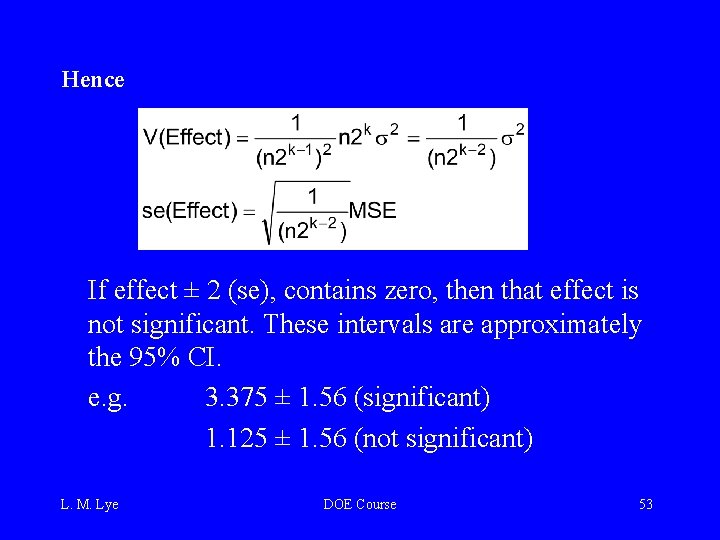
Hence If effect ± 2 (se), contains zero, then that effect is not significant. These intervals are approximately the 95% CI. e. g. 3. 375 ± 1. 56 (significant) 1. 125 ± 1. 56 (not significant) L. M. Lye DOE Course 53

c) Normal probability plot of effects Significant effects are those that do not fit on normal probability plot. i. e. non-significant effects will lie along the line of a normal probability plot of the effects. Good visual tool - available in Design-Expert software. L. M. Lye DOE Course 54

Design and Analysis of Multi-Factored Experiments Examples of Computer Analysis L. M. Lye DOE Course 55

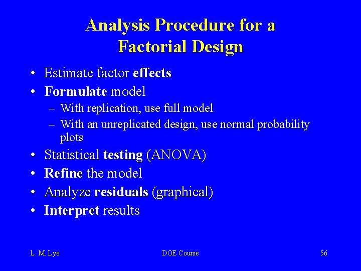
Analysis Procedure for a Factorial Design • Estimate factor effects • Formulate model – With replication, use full model – With an unreplicated design, use normal probability plots • • Statistical testing (ANOVA) Refine the model Analyze residuals (graphical) Interpret results L. M. Lye DOE Course 56

Chemical Process Example A = reactant concentration, B = catalyst amount, y = recovery L. M. Lye DOE Course 57

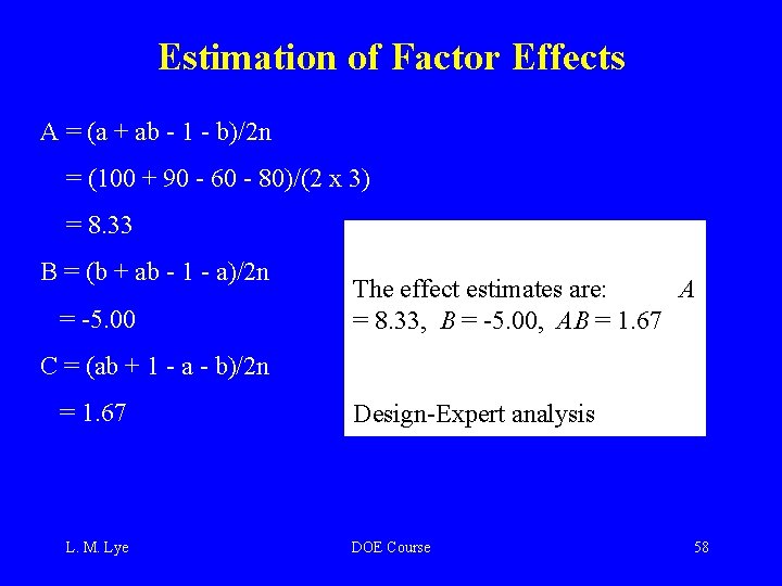
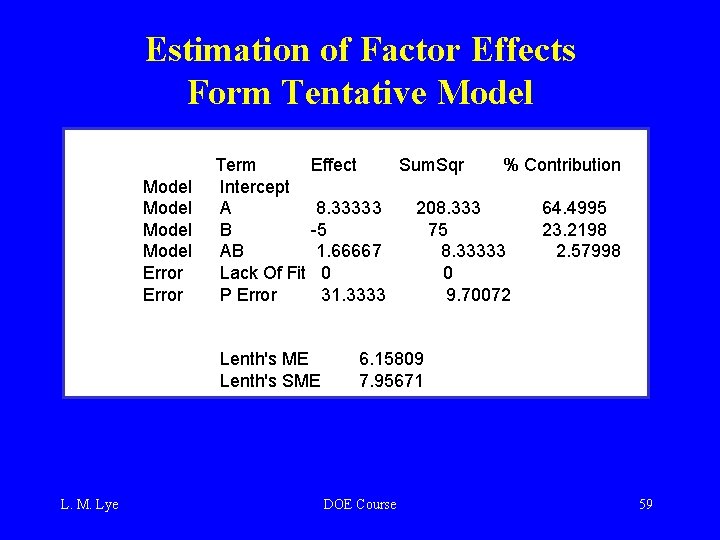
Estimation of Factor Effects A = (a + ab - 1 - b)/2 n = (100 + 90 - 60 - 80)/(2 x 3) = 8. 33 B = (b + ab - 1 - a)/2 n = -5. 00 The effect estimates are: A = 8. 33, B = -5. 00, AB = 1. 67 C = (ab + 1 - a - b)/2 n = 1. 67 L. M. Lye Design-Expert analysis DOE Course 58

Estimation of Factor Effects Form Tentative Model Model Error Term Effect Sum. Sqr % Contribution Intercept A 8. 33333 208. 333 64. 4995 B -5 75 23. 2198 AB 1. 66667 8. 33333 2. 57998 Lack Of Fit 0 0 P Error 31. 3333 9. 70072 Lenth's ME Lenth's SME L. M. Lye 6. 15809 7. 95671 DOE Course 59

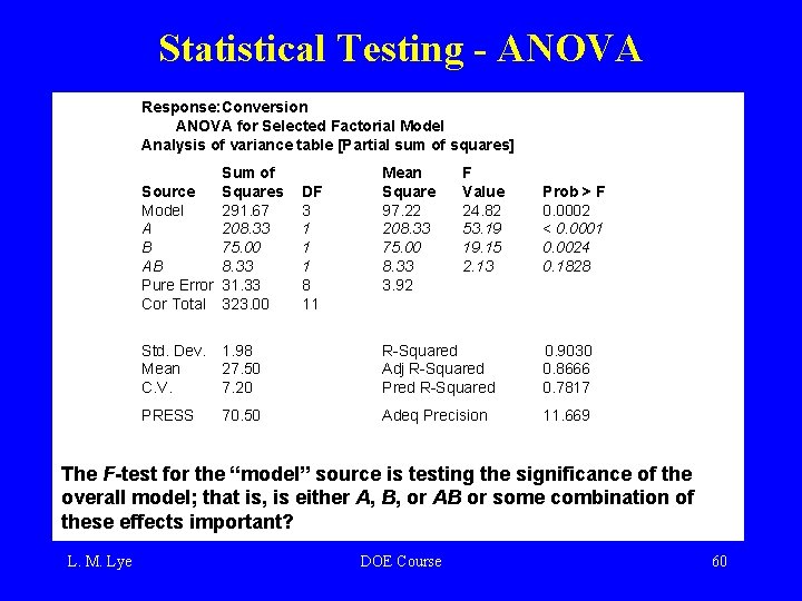
Statistical Testing - ANOVA Response: Conversion ANOVA for Selected Factorial Model Analysis of variance table [Partial sum of squares] Sum of Source Squares Model 291. 67 A 208. 33 B 75. 00 AB 8. 33 Pure Error 31. 33 Cor Total 323. 00 DF 3 1 1 1 8 11 Mean Square 97. 22 208. 33 75. 00 8. 33 3. 92 F Value 24. 82 53. 19 19. 15 2. 13 Prob > F 0. 0002 < 0. 0001 0. 0024 0. 1828 Std. Dev. Mean C. V. 1. 98 27. 50 7. 20 R-Squared Adj R-Squared Pred R-Squared 0. 9030 0. 8666 0. 7817 PRESS 70. 50 Adeq Precision 11. 669 The F-test for the “model” source is testing the significance of the overall model; that is, is either A, B, or AB or some combination of these effects important? L. M. Lye DOE Course 60

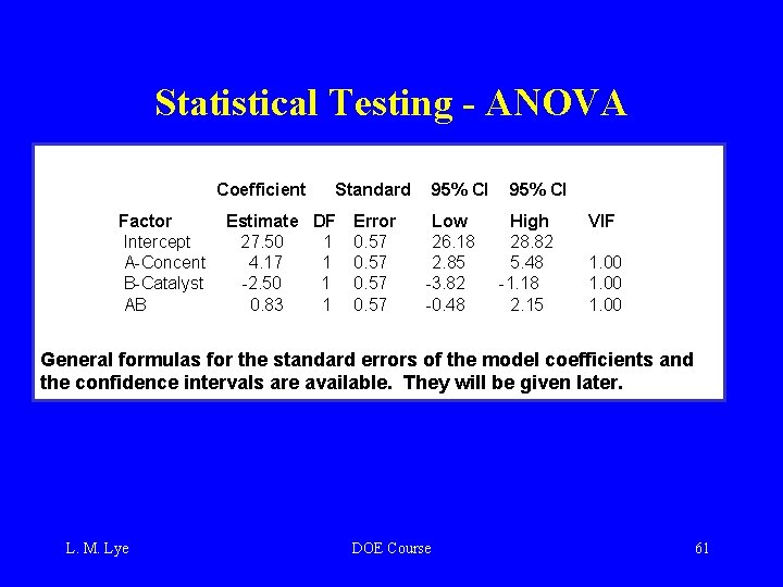
Statistical Testing - ANOVA Coefficient Factor Intercept A-Concent B-Catalyst AB Standard Estimate DF Error 27. 50 1 0. 57 4. 17 1 0. 57 -2. 50 1 0. 57 0. 83 1 0. 57 95% CI Low 26. 18 2. 85 -3. 82 -0. 48 95% CI High 28. 82 5. 48 -1. 18 2. 15 VIF 1. 00 General formulas for the standard errors of the model coefficients and the confidence intervals are available. They will be given later. L. M. Lye DOE Course 61

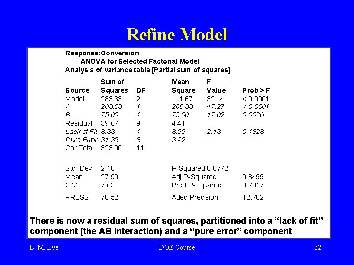
Refine Model Response: Conversion ANOVA for Selected Factorial Model Analysis of variance table [Partial sum of squares] Sum of Source Squares Model 283. 33 A 208. 33 B 75. 00 Residual 39. 67 Lack of Fit 8. 33 Pure Error 31. 33 Cor Total 323. 00 DF 2 1 1 9 1 8 11 Mean Square 141. 67 208. 33 75. 00 4. 41 8. 33 3. 92 F Value 32. 14 47. 27 17. 02 Prob > F < 0. 0001 0. 0026 2. 13 0. 1828 Std. Dev. Mean C. V. 2. 10 27. 50 7. 63 R-Squared 0. 8772 Adj R-Squared Pred R-Squared 0. 8499 0. 7817 PRESS 70. 52 Adeq Precision 12. 702 There is now a residual sum of squares, partitioned into a “lack of fit” component (the AB interaction) and a “pure error” component L. M. Lye DOE Course 62

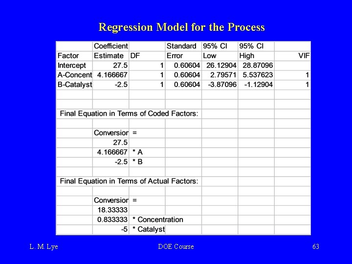
Regression Model for the Process L. M. Lye DOE Course 63

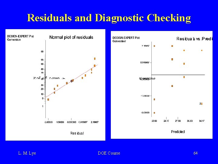
Residuals and Diagnostic Checking L. M. Lye DOE Course 64

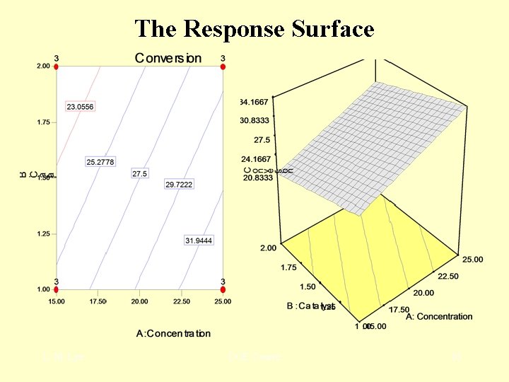
The Response Surface L. M. Lye DOE Course 65

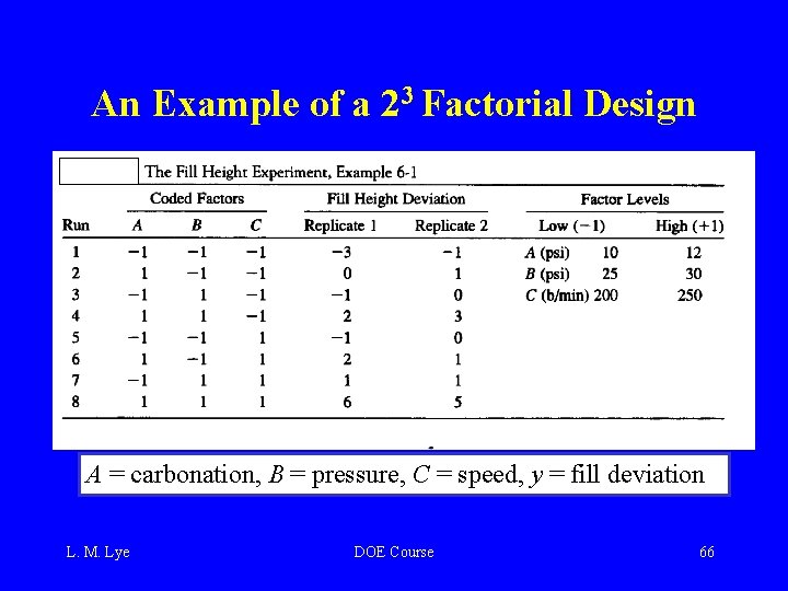
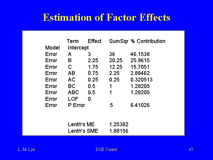
An Example of a 23 Factorial Design A = carbonation, B = pressure, C = speed, y = fill deviation L. M. Lye DOE Course 66

Estimation of Factor Effects Model Error Error Error L. M. Lye Term Effect Intercept A 3 B 2. 25 C 1. 75 AB 0. 75 AC 0. 25 BC 0. 5 ABC 0. 5 LOF 0 P Error Sum. Sqr % Contribution Lenth's ME Lenth's SME 1. 25382 1. 88156 36 20. 25 12. 25 0. 25 1 1 46. 1538 25. 9615 15. 7051 2. 88462 0. 320513 1. 28205 5 6. 41026 DOE Course 67

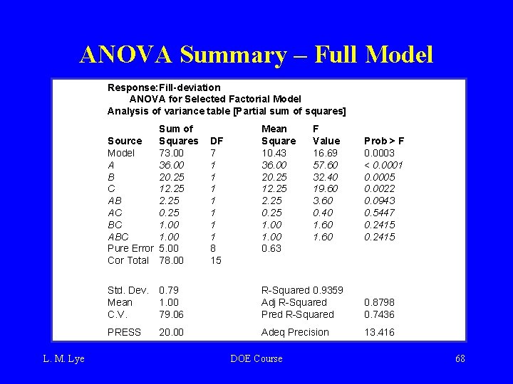
ANOVA Summary – Full Model Response: Fill-deviation ANOVA for Selected Factorial Model Analysis of variance table [Partial sum of squares] Sum of Source Squares Model 73. 00 A 36. 00 B 20. 25 C 12. 25 AB 2. 25 AC 0. 25 BC 1. 00 ABC 1. 00 Pure Error 5. 00 Cor Total 78. 00 L. M. Lye DF 7 1 1 1 1 8 15 Mean Square 10. 43 36. 00 20. 25 12. 25 0. 25 1. 00 0. 63 F Value 16. 69 57. 60 32. 40 19. 60 3. 60 0. 40 1. 60 Prob > F 0. 0003 < 0. 0001 0. 0005 0. 0022 0. 0943 0. 5447 0. 2415 Std. Dev. Mean C. V. 0. 79 1. 00 79. 06 R-Squared 0. 9359 Adj R-Squared Pred R-Squared 0. 8798 0. 7436 PRESS 20. 00 Adeq Precision 13. 416 DOE Course 68

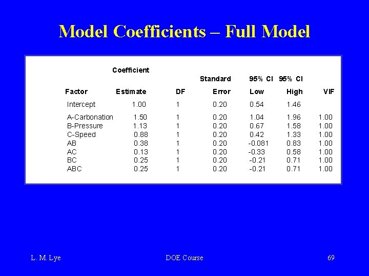
Model Coefficients – Full Model Coefficient Standard Factor L. M. Lye Estimate 95% CI DF Error Low High Intercept 1. 00 1 0. 20 0. 54 1. 46 A-Carbonation B-Pressure C-Speed AB AC BC ABC 1. 50 1. 13 0. 88 0. 38 0. 13 0. 25 1 1 1 1 0. 20 0. 20 1. 04 0. 67 0. 42 -0. 081 -0. 33 -0. 21 1. 96 1. 58 1. 33 0. 83 0. 58 0. 71 DOE Course VIF 1. 00 1. 00 69

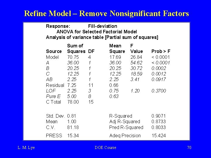
Refine Model – Remove Nonsignificant Factors Response: Fill-deviation ANOVA for Selected Factorial Model Analysis of variance table [Partial sum of squares] Sum of Source Squares Model 70. 75 A 36. 00 B 20. 25 C 12. 25 AB 2. 25 Residual 7. 25 LOF 2. 25 Pure E 5. 00 C Total 78. 00 L. M. Lye DF 4 1 1 11 3 8 15 Mean Square 17. 69 36. 00 20. 25 12. 25 0. 66 0. 75 0. 63 F Value 26. 84 54. 62 30. 72 18. 59 3. 41 Prob > F < 0. 0001 0. 0002 0. 0012 0. 0917 1. 20 0. 3700 Std. Dev. 0. 81 Mean 1. 00 C. V. 81. 18 R-Squared Adj R-Squared Pred R-Squared 0. 9071 0. 8733 0. 8033 PRESS Adeq Precision 15. 424 15. 34 DOE Course 70

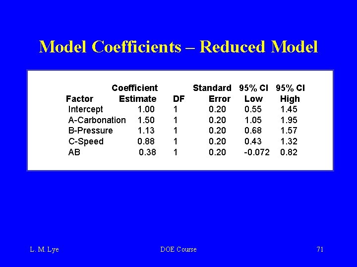
Model Coefficients – Reduced Model Coefficient Factor Estimate Intercept 1. 00 A-Carbonation 1. 50 B-Pressure 1. 13 C-Speed 0. 88 AB 0. 38 L. M. Lye Standard 95% CI DF Error Low High 1 0. 20 0. 55 1. 45 1 0. 20 1. 05 1. 95 1 0. 20 0. 68 1. 57 1 0. 20 0. 43 1. 32 1 0. 20 -0. 072 0. 82 DOE Course 71

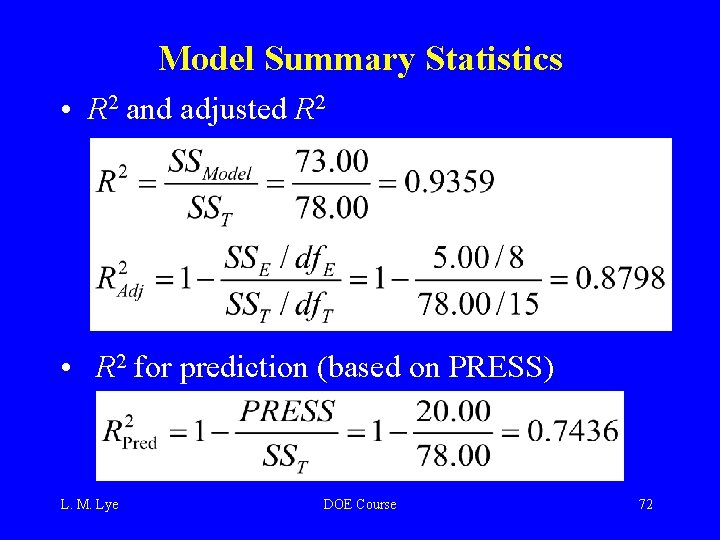
Model Summary Statistics • R 2 and adjusted R 2 • R 2 for prediction (based on PRESS) L. M. Lye DOE Course 72

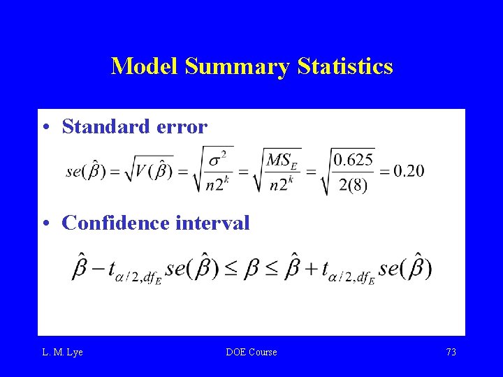
Model Summary Statistics • Standard error of model coefficients • Confidence interval on model coefficients L. M. Lye DOE Course 73

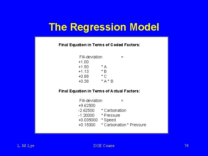
The Regression Model Final Equation in Terms of Coded Factors: Fill-deviation +1. 00 +1. 50 *A +1. 13 *B +0. 88 *C +0. 38 *A*B = Final Equation in Terms of Actual Factors: Fill-deviation = +9. 62500 -2. 62500 * Carbonation -1. 20000 * Pressure +0. 035000 * Speed +0. 15000 * Carbonation * Pressure L. M. Lye DOE Course 74

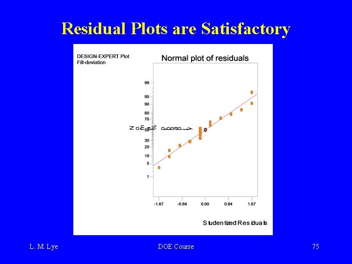
Residual Plots are Satisfactory L. M. Lye DOE Course 75

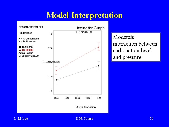
Model Interpretation Moderate interaction between carbonation level and pressure L. M. Lye DOE Course 76

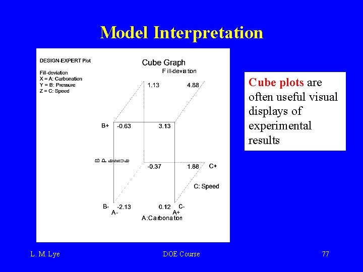
Model Interpretation Cube plots are often useful visual displays of experimental results L. M. Lye DOE Course 77

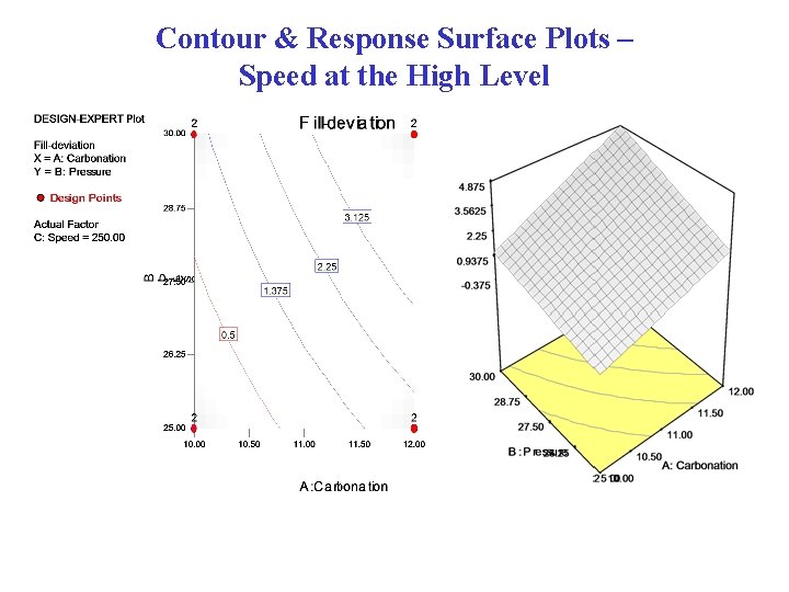
Contour & Response Surface Plots – Speed at the High Level L. M. Lye DOE Course 78

Design and Analysis of Multi-Factored Experiments Unreplicated Factorials L. M. Lye DOE Course 79

Unreplicated 2 k Factorial Designs • These are 2 k factorial designs with one observation at each corner of the “cube” • An unreplicated 2 k factorial design is also sometimes called a “single replicate” of the 2 k • These designs are very widely used • Risks…if there is only one observation at each corner, is there a chance of unusual response observations spoiling the results? • Modeling “noise”? L. M. Lye DOE Course 80

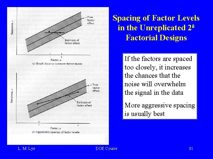
Spacing of Factor Levels in the Unreplicated 2 k Factorial Designs If the factors are spaced too closely, it increases the chances that the noise will overwhelm the signal in the data More aggressive spacing is usually best L. M. Lye DOE Course 81

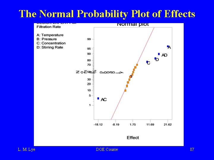
Unreplicated 2 k Factorial Designs • Lack of replication causes potential problems in statistical testing – Replication admits an estimate of “pure error” (a better phrase is an internal estimate of error) – With no replication, fitting the full model results in zero degrees of freedom for error • Potential solutions to this problem – Pooling high-order interactions to estimate error – Normal probability plotting of effects (Daniels, 1959) L. M. Lye DOE Course 82

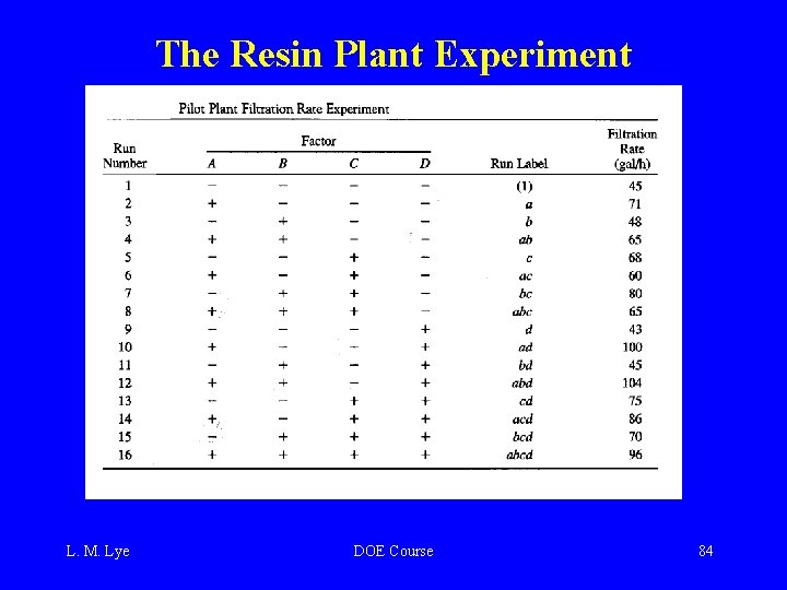
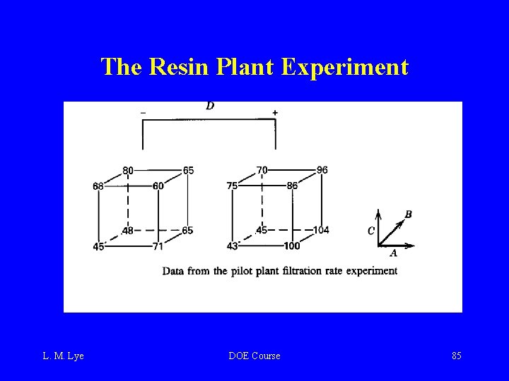
Example of an Unreplicated 2 k Design • A 24 factorial was used to investigate the effects of four factors on the filtration rate of a resin • The factors are A = temperature, B = pressure, C = mole ratio, D= stirring rate • Experiment was performed in a pilot plant L. M. Lye DOE Course 83

The Resin Plant Experiment L. M. Lye DOE Course 84

The Resin Plant Experiment L. M. Lye DOE Course 85

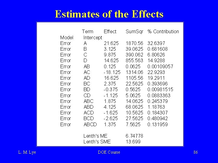
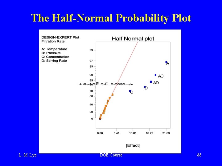
Estimates of the Effects Model Error Error Error Error Term Intercept A B C D AB AC AD BC BD CD ABC ABD ACD BCD ABCD Effect Sum. Sqr % Contribution 21. 625 3. 125 9. 875 14. 625 0. 125 -18. 125 16. 625 2. 375 -0. 375 -1. 125 1. 875 4. 125 -1. 625 -2. 625 1. 375 1870. 56 39. 0625 390. 062 855. 563 0. 0625 1314. 06 1105. 56 22. 5625 0. 5625 5. 0625 14. 0625 68. 0625 10. 5625 27. 5625 Lenth's ME Lenth's SME L. M. Lye DOE Course 32. 6397 0. 681608 6. 80626 14. 9288 0. 00109057 22. 9293 19. 2911 0. 393696 0. 00981515 0. 0883363 0. 245379 1. 18763 0. 184307 0. 480942 0. 131959 6. 74778 13. 699 86

The Normal Probability Plot of Effects L. M. Lye DOE Course 87

The Half-Normal Probability Plot L. M. Lye DOE Course 88

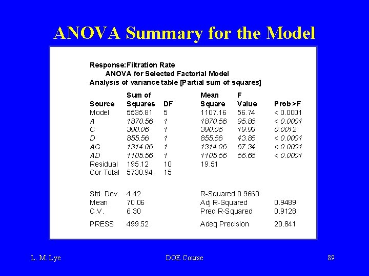
ANOVA Summary for the Model Response: Filtration Rate ANOVA for Selected Factorial Model Analysis of variance table [Partial sum of squares] L. M. Lye Source Model A C D AC AD Residual Cor Total Sum of Squares 5535. 81 1870. 56 390. 06 855. 56 1314. 06 1105. 56 195. 12 5730. 94 Std. Dev. Mean C. V. 4. 42 70. 06 6. 30 R-Squared 0. 9660 Adj R-Squared Pred R-Squared 0. 9489 0. 9128 PRESS 499. 52 Adeq Precision 20. 841 DF 5 1 1 10 15 Mean Square 1107. 16 1870. 56 390. 06 855. 56 1314. 06 1105. 56 19. 51 DOE Course F Value 56. 74 95. 86 19. 99 43. 85 67. 34 56. 66 Prob >F < 0. 0001 0. 0012 < 0. 0001 89

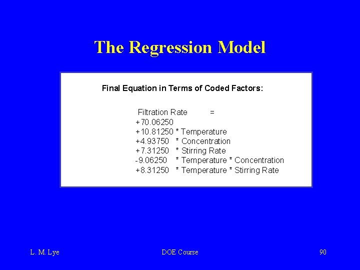
The Regression Model Final Equation in Terms of Coded Factors: Filtration Rate = +70. 06250 +10. 81250 * Temperature +4. 93750 * Concentration +7. 31250 * Stirring Rate -9. 06250 * Temperature * Concentration +8. 31250 * Temperature * Stirring Rate L. M. Lye DOE Course 90

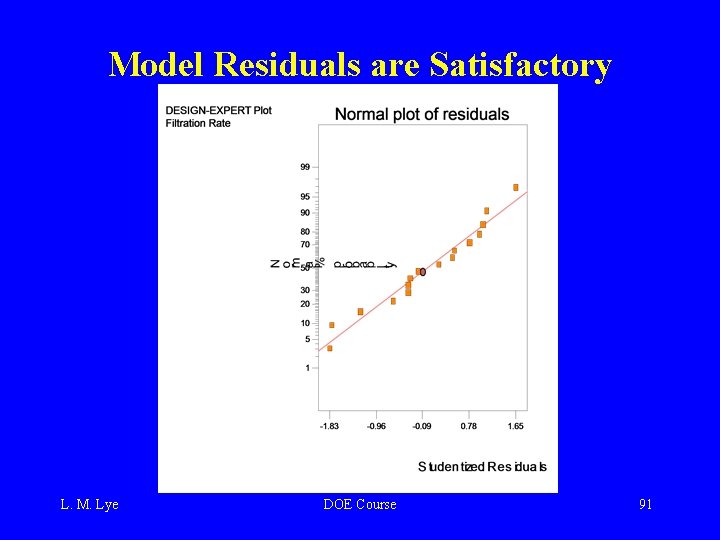
Model Residuals are Satisfactory L. M. Lye DOE Course 91

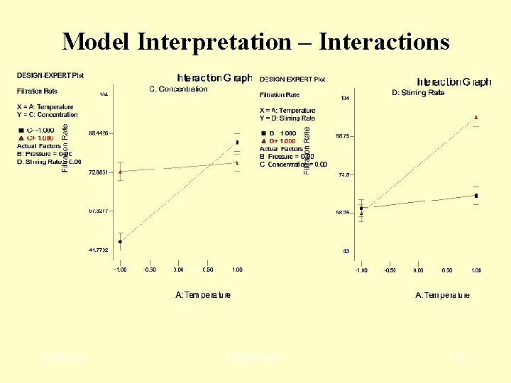
Model Interpretation – Interactions L. M. Lye DOE Course 92

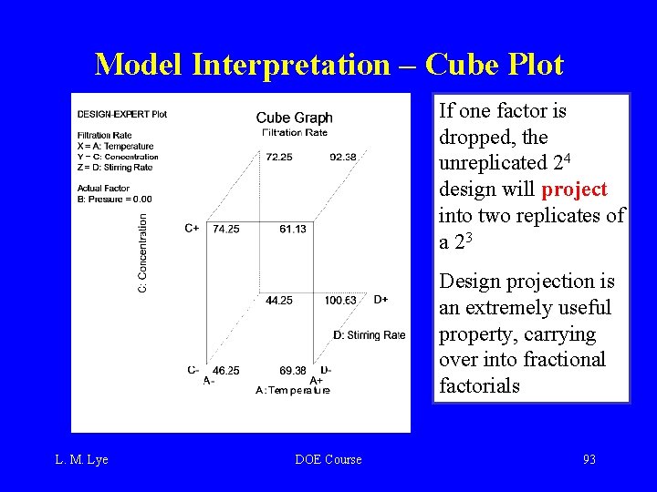
Model Interpretation – Cube Plot If one factor is dropped, the unreplicated 24 design will project into two replicates of a 23 Design projection is an extremely useful property, carrying over into fractional factorials L. M. Lye DOE Course 93

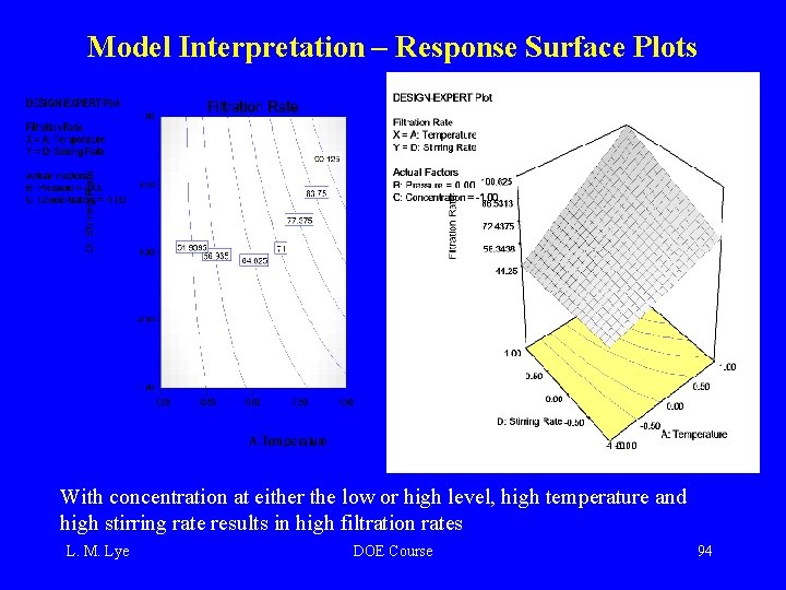
Model Interpretation – Response Surface Plots With concentration at either the low or high level, high temperature and high stirring rate results in high filtration rates L. M. Lye DOE Course 94

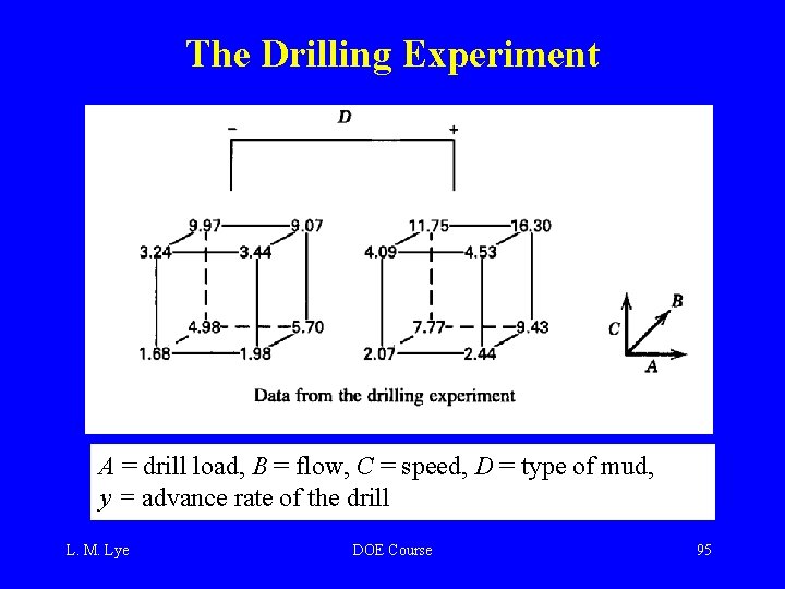
The Drilling Experiment A = drill load, B = flow, C = speed, D = type of mud, y = advance rate of the drill L. M. Lye DOE Course 95

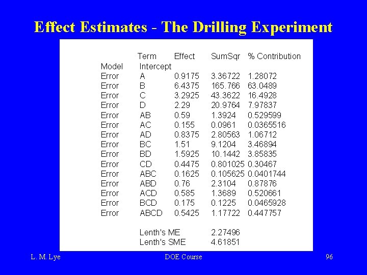
Effect Estimates - The Drilling Experiment Model Error Error Error Error Term Intercept A B C D AB AC AD BC BD CD ABC ABD ACD BCD ABCD Effect Sum. Sqr % Contribution 0. 9175 6. 4375 3. 2925 2. 29 0. 59 0. 155 0. 8375 1. 51 1. 5925 0. 4475 0. 1625 0. 76 0. 585 0. 175 0. 5425 3. 36722 165. 766 43. 3622 20. 9764 1. 3924 0. 0961 2. 80563 9. 1204 10. 1442 0. 801025 0. 105625 2. 3104 1. 3689 0. 1225 1. 17722 Lenth's ME Lenth's SME L. M. Lye DOE Course 1. 28072 63. 0489 16. 4928 7. 97837 0. 529599 0. 0365516 1. 06712 3. 46894 3. 85835 0. 30467 0. 0401744 0. 87876 0. 520661 0. 0465928 0. 447757 2. 27496 4. 61851 96

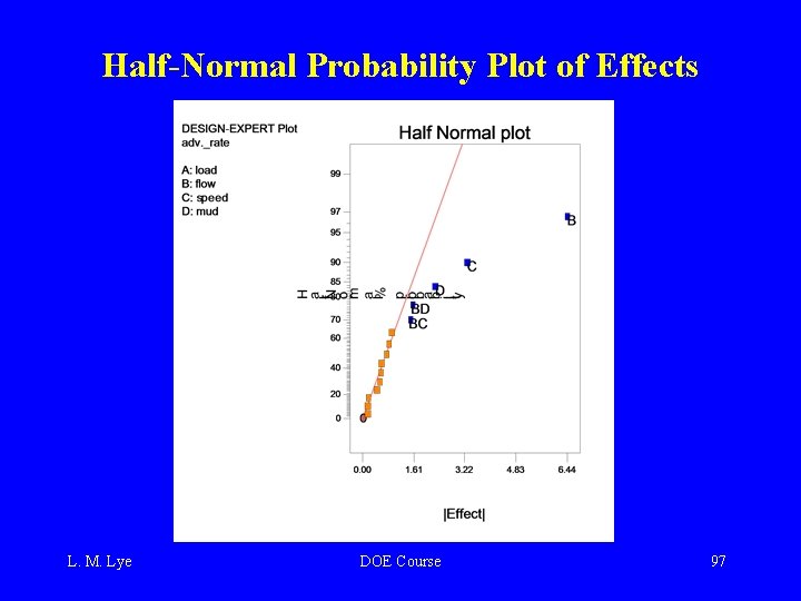
Half-Normal Probability Plot of Effects L. M. Lye DOE Course 97

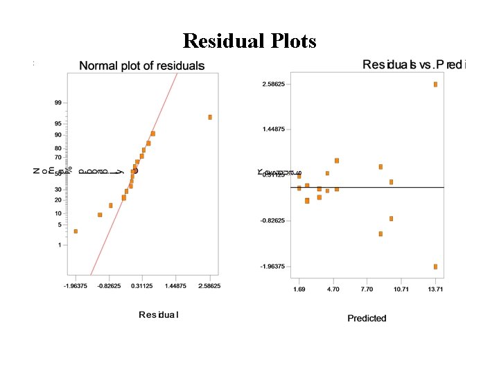
Residual Plots L. M. Lye DOE Course 98

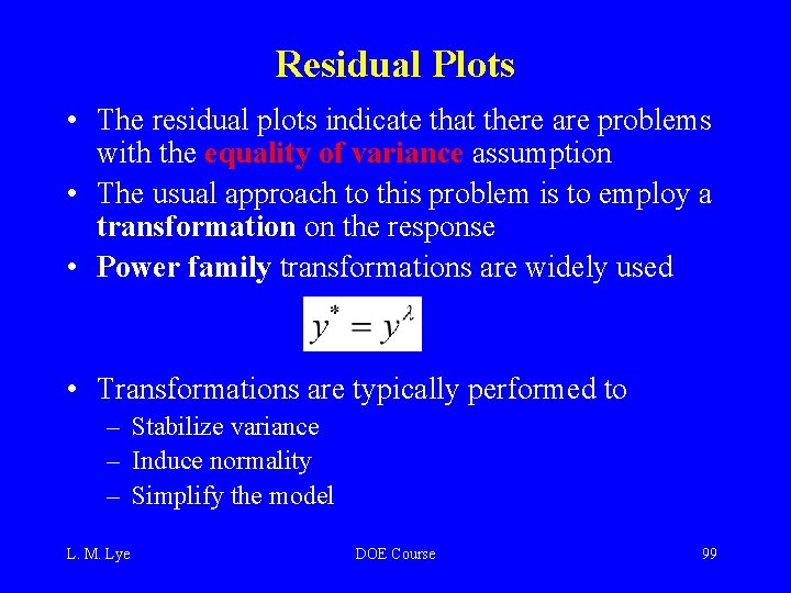
Residual Plots • The residual plots indicate that there are problems with the equality of variance assumption • The usual approach to this problem is to employ a transformation on the response • Power family transformations are widely used • Transformations are typically performed to – Stabilize variance – Induce normality – Simplify the model L. M. Lye DOE Course 99

Selecting a Transformation • Empirical selection of lambda • Prior (theoretical) knowledge or experience can often suggest the form of a transformation • Analytical selection of lambda…the Box-Cox (1964) method (simultaneously estimates the model parameters and the transformation parameter lambda) • Box-Cox method implemented in Design-Expert L. M. Lye DOE Course 100

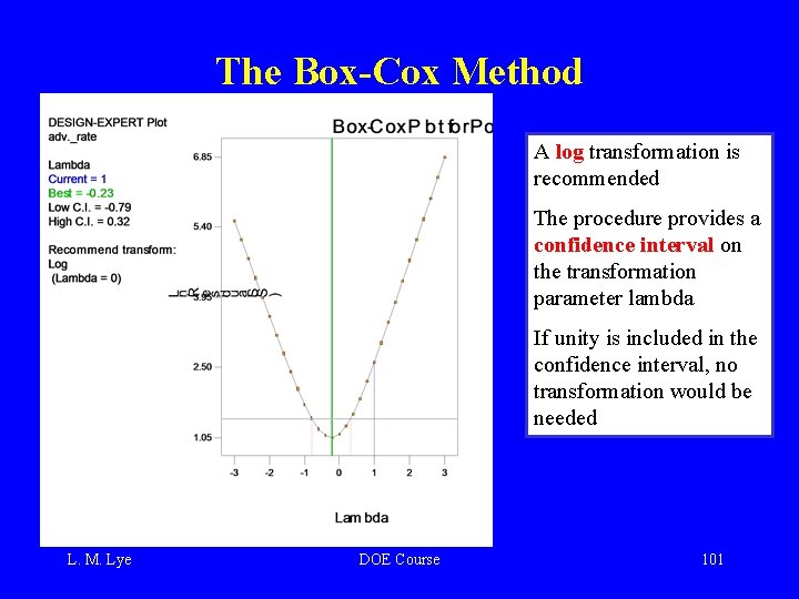
The Box-Cox Method A log transformation is recommended The procedure provides a confidence interval on the transformation parameter lambda If unity is included in the confidence interval, no transformation would be needed L. M. Lye DOE Course 101

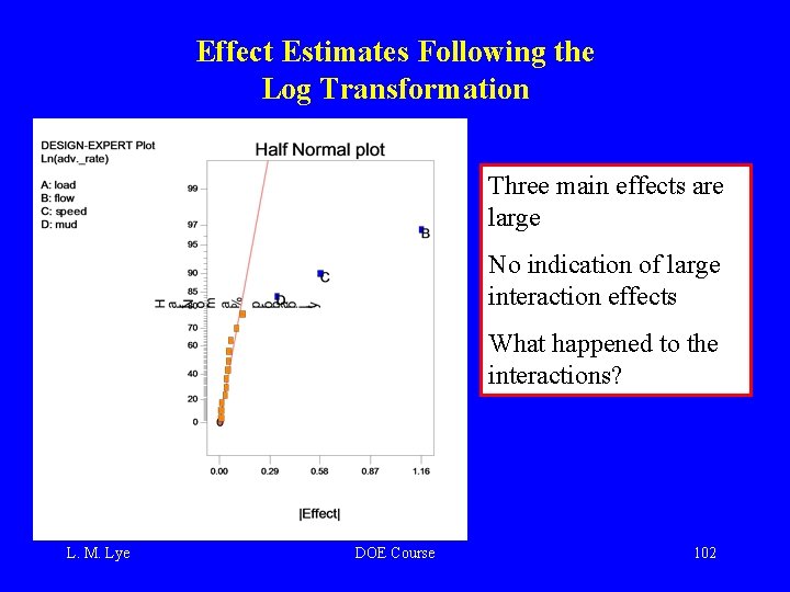
Effect Estimates Following the Log Transformation Three main effects are large No indication of large interaction effects What happened to the interactions? L. M. Lye DOE Course 102

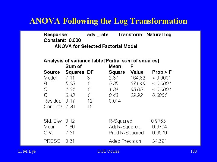
ANOVA Following the Log Transformation Response: adv. _rate Transform: Natural log Constant: 0. 000 ANOVA for Selected Factorial Model Analysis of variance table [Partial sum of squares] Sum of Mean F Source Squares DF Square Value Prob > F Model 7. 11 3 2. 37 164. 82 < 0. 0001 B 5. 35 1 5. 35 371. 49 < 0. 0001 C 1. 34 1 1. 34 93. 05 < 0. 0001 D 0. 43 1 0. 43 29. 92 0. 0001 Residual 0. 17 12 0. 014 Cor Total 7. 29 15 L. M. Lye Std. Dev. 0. 12 Mean 1. 60 C. V. 7. 51 R-Squared Adj R-Squared Pred R-Squared 0. 9763 0. 9704 0. 9579 PRESS Adeq Precision 34. 391 0. 31 DOE Course 103

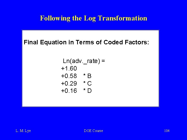
Following the Log Transformation Final Equation in Terms of Coded Factors: Ln(adv. _rate) = +1. 60 +0. 58 * B +0. 29 * C +0. 16 * D L. M. Lye DOE Course 104

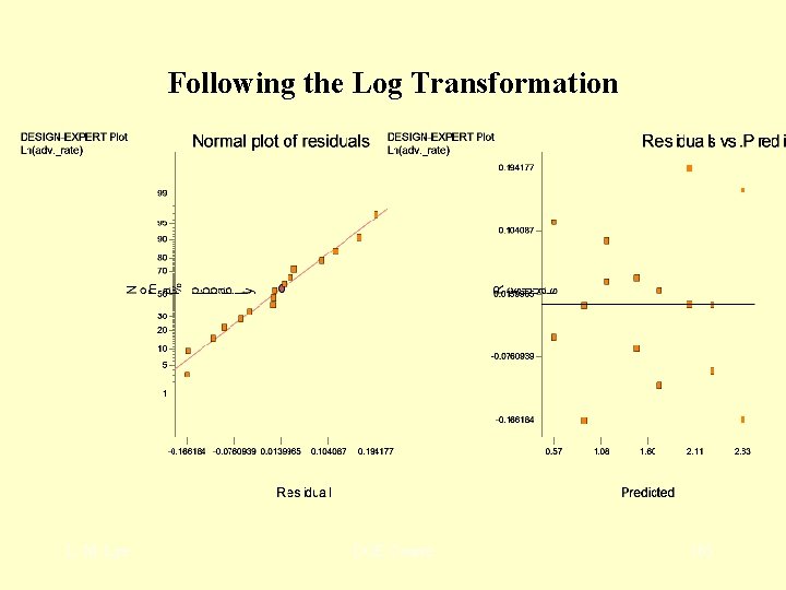
Following the Log Transformation L. M. Lye DOE Course 105

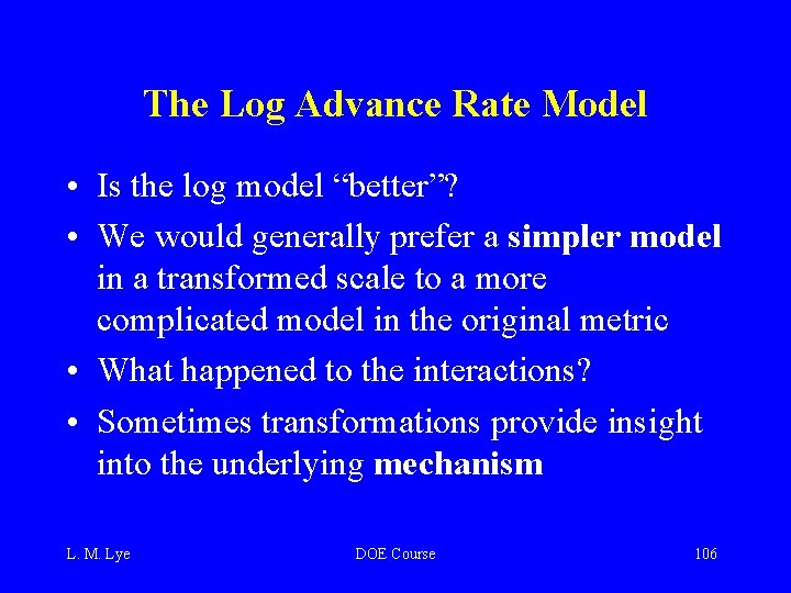
The Log Advance Rate Model • Is the log model “better”? • We would generally prefer a simpler model in a transformed scale to a more complicated model in the original metric • What happened to the interactions? • Sometimes transformations provide insight into the underlying mechanism L. M. Lye DOE Course 106

Other Analysis Methods for Unreplicated 2 k Designs • Lenth’s method – Analytical method for testing effects, uses an estimate of error formed by pooling small contrasts – Some adjustment to the critical values in the original method can be helpful – Probably most useful as a supplement to the normal probability plot L. M. Lye DOE Course 107

Design and Analysis of Multi-Factored Experiments Center points L. M. Lye DOE Course 108

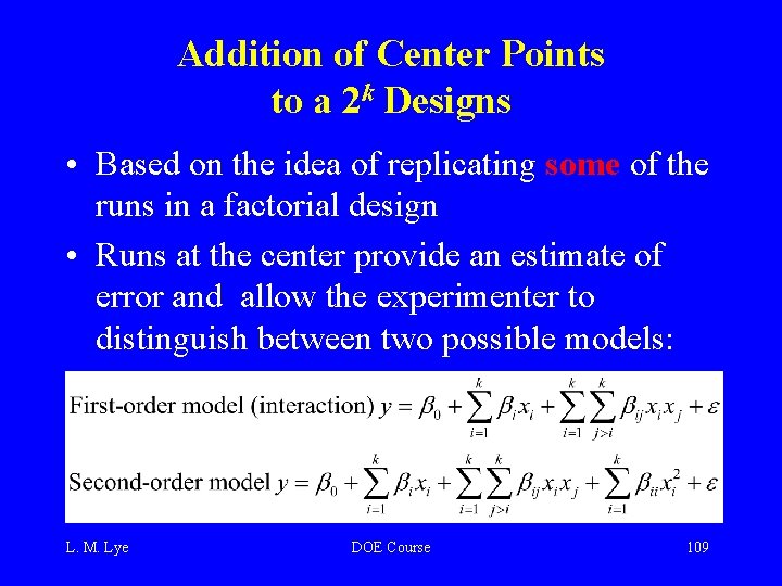
Addition of Center Points to a 2 k Designs • Based on the idea of replicating some of the runs in a factorial design • Runs at the center provide an estimate of error and allow the experimenter to distinguish between two possible models: L. M. Lye DOE Course 109

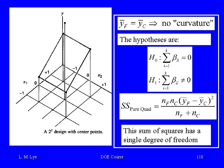
The hypotheses are: This sum of squares has a single degree of freedom L. M. Lye DOE Course 110

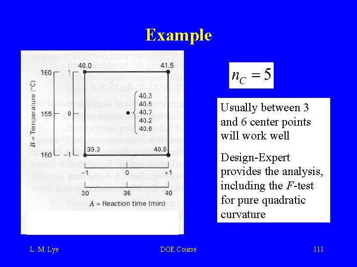
Example Usually between 3 and 6 center points will work well Design-Expert provides the analysis, including the F-test for pure quadratic curvature L. M. Lye DOE Course 111

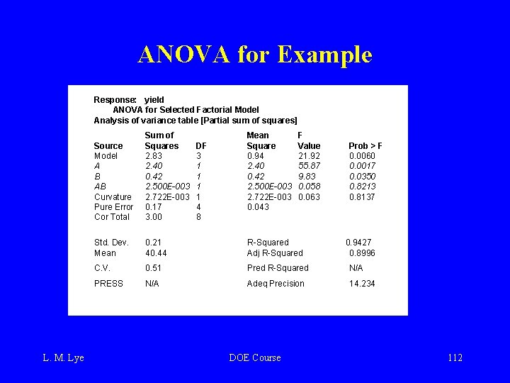
ANOVA for Example Response: yield ANOVA for Selected Factorial Model Analysis of variance table [Partial sum of squares] L. M. Lye Source Model A B AB Curvature Pure Error Cor Total Sum of Squares 2. 83 2. 40 0. 42 2. 500 E-003 2. 722 E-003 0. 17 3. 00 Std. Dev. Mean 0. 21 40. 44 R-Squared Adj R-Squared C. V. 0. 51 Pred R-Squared N/A PRESS N/A Adeq Precision 14. 234 DF 3 1 1 4 8 Mean Square 0. 94 2. 40 0. 42 2. 500 E-003 2. 722 E-003 0. 043 DOE Course F Value 21. 92 55. 87 9. 83 0. 058 0. 063 Prob > F 0. 0060 0. 0017 0. 0350 0. 8213 0. 8137 0. 9427 0. 8996 112

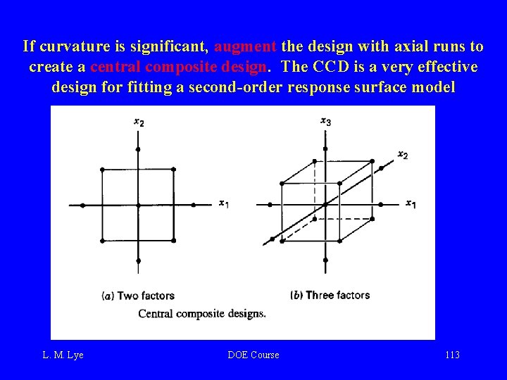
If curvature is significant, augment the design with axial runs to create a central composite design. The CCD is a very effective design for fitting a second-order response surface model L. M. Lye DOE Course 113

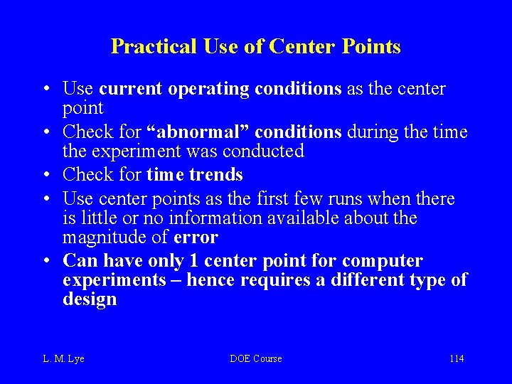
Practical Use of Center Points • Use current operating conditions as the center point • Check for “abnormal” conditions during the time the experiment was conducted • Check for time trends • Use center points as the first few runs when there is little or no information available about the magnitude of error • Can have only 1 center point for computer experiments – hence requires a different type of design L. M. Lye DOE Course 114