DATA MINING LECTURE 7 Dimensionality Reduction PCA SVD

DATA MINING LECTURE 7 Dimensionality Reduction PCA – SVD (Thanks to Jure Leskovec, Evimaria Terzi)

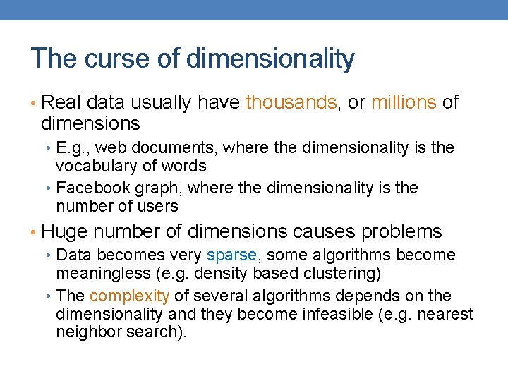
The curse of dimensionality • Real data usually have thousands, or millions of dimensions • E. g. , web documents, where the dimensionality is the vocabulary of words • Facebook graph, where the dimensionality is the number of users • Huge number of dimensions causes problems • Data becomes very sparse, some algorithms become meaningless (e. g. density based clustering) • The complexity of several algorithms depends on the dimensionality and they become infeasible (e. g. nearest neighbor search).

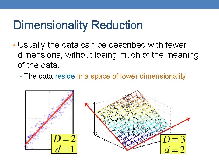
Dimensionality Reduction • Usually the data can be described with fewer dimensions, without losing much of the meaning of the data. • The data reside in a space of lower dimensionality

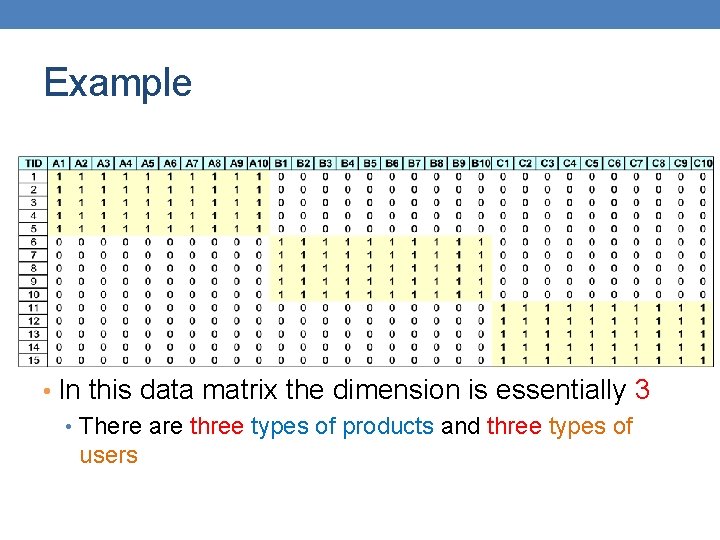
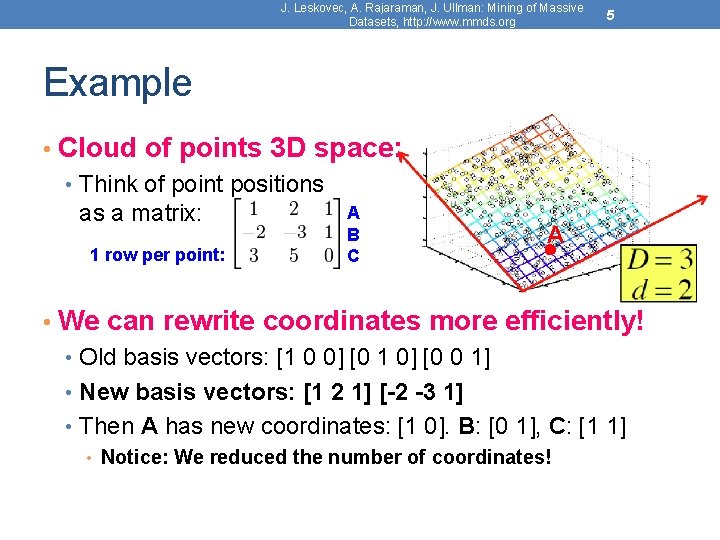
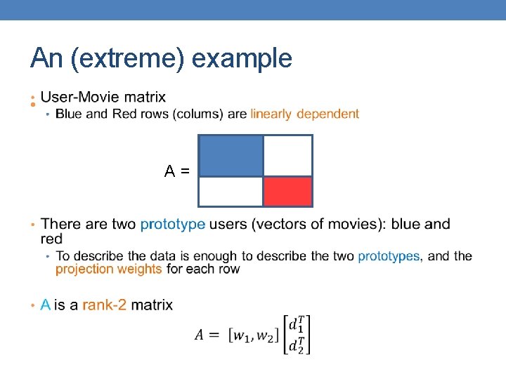
Example • In this data matrix the dimension is essentially 3 • There are three types of products and three types of users

J. Leskovec, A. Rajaraman, J. Ullman: Mining of Massive Datasets, http: //www. mmds. org 5 Example • Cloud of points 3 D space: • Think of point positions A as a matrix: 1 row per point: B C A • We can rewrite coordinates more efficiently! • Old basis vectors: [1 0 0] [0 1 0] [0 0 1] • New basis vectors: [1 2 1] [-2 -3 1] • Then A has new coordinates: [1 0]. B: [0 1], C: [1 1] • Notice: We reduced the number of coordinates!

Dimensionality Reduction • Find the “true dimension” of the data • In reality things are never as clear and simple as in this example, but we can still reduce the dimension. • Essentially, we assume that some of the data is noise, and we can approximate the useful part with a lower dimensionality space. • Dimensionality reduction does not just reduce the amount of data, it often brings out the useful part of the data

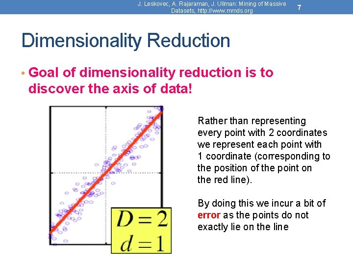
J. Leskovec, A. Rajaraman, J. Ullman: Mining of Massive Datasets, http: //www. mmds. org 7 Dimensionality Reduction • Goal of dimensionality reduction is to discover the axis of data! Rather than representing every point with 2 coordinates we represent each point with 1 coordinate (corresponding to the position of the point on the red line). By doing this we incur a bit of error as the points do not exactly lie on the line

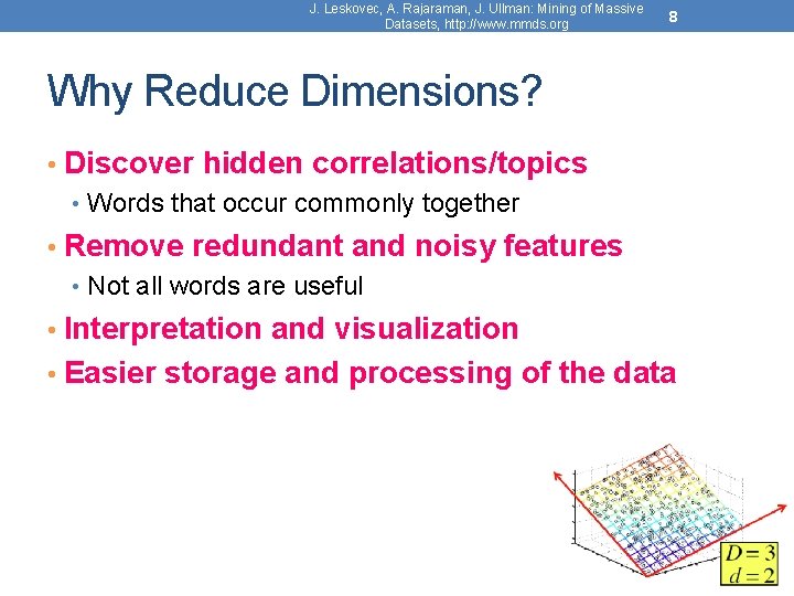
J. Leskovec, A. Rajaraman, J. Ullman: Mining of Massive Datasets, http: //www. mmds. org 8 Why Reduce Dimensions? • Discover hidden correlations/topics • Words that occur commonly together • Remove redundant and noisy features • Not all words are useful • Interpretation and visualization • Easier storage and processing of the data

Dimensionality Reduction • We have already seen a form of dimensionality reduction • LSH, and random projections reduce the dimension while preserving the distances

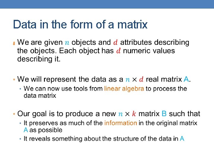
Data in the form of a matrix •

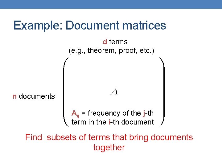
Example: Document matrices d terms (e. g. , theorem, proof, etc. ) n documents Aij = frequency of the j-th term in the i-th document Find subsets of terms that bring documents together

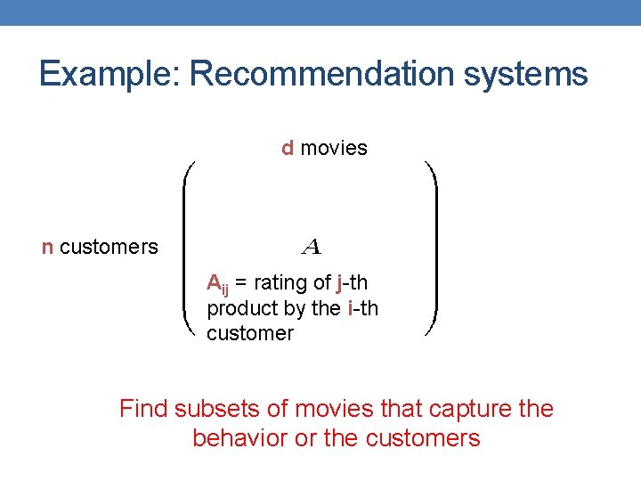
Example: Recommendation systems d movies n customers Aij = rating of j-th product by the i-th customer Find subsets of movies that capture the behavior or the customers

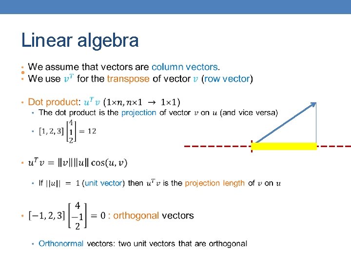
Linear algebra •

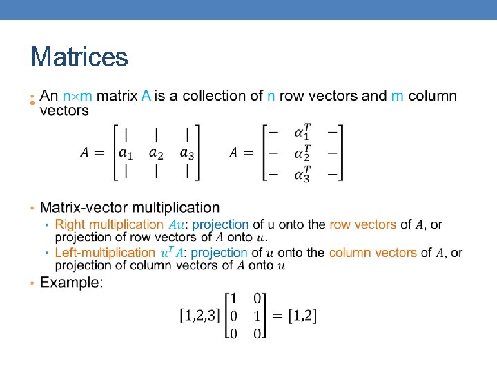
Matrices •

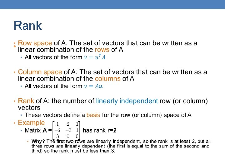
Rank •

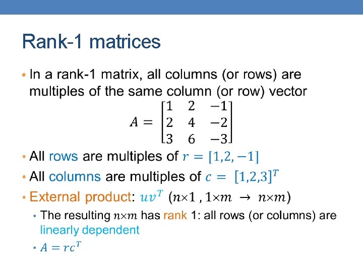
Rank-1 matrices •

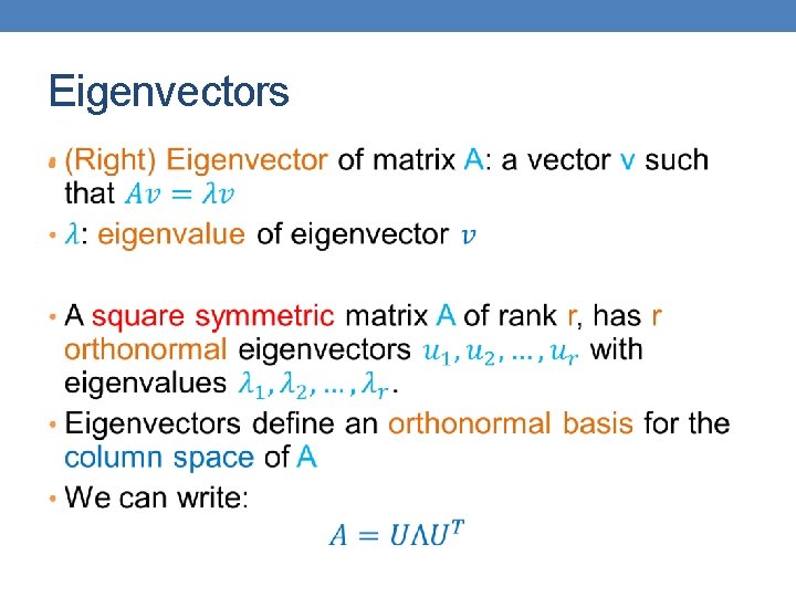
Eigenvectors •

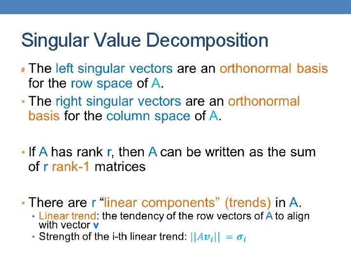
Singular Value Decomposition • [n×m] = [n×r] [r×m] r: rank of matrix A

Singular Value Decomposition •

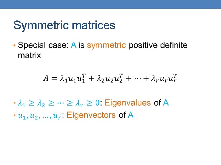
Symmetric matrices •

An (extreme) example • A=

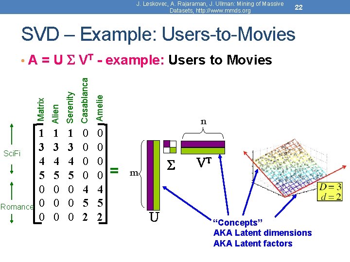
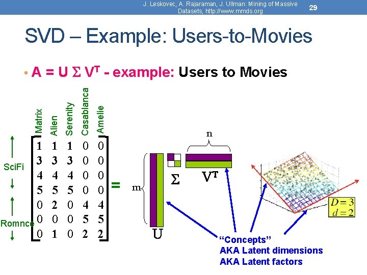
J. Leskovec, A. Rajaraman, J. Ullman: Mining of Massive Datasets, http: //www. mmds. org 22 SVD – Example: Users-to-Movies Serenity Casablanca Amelie Romance Alien Sci. Fi Matrix • A = U VT - example: Users to Movies 1 3 4 5 0 0 0 0 4 5 2 0 0 4 5 2 n = m U VT “Concepts” AKA Latent dimensions AKA Latent factors

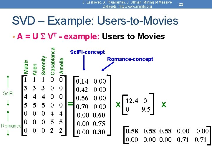
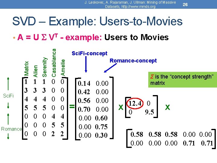
J. Leskovec, A. Rajaraman, J. Ullman: Mining of Massive Datasets, http: //www. mmds. org 23 SVD – Example: Users-to-Movies Serenity Casablanca Amelie Romance Alien Sci. Fi Matrix • A = U VT - example: Users to Movies 1 3 4 5 0 0 0 0 4 5 2 0 0 4 5 2 Sci. Fi-concept Romance-concept = 0. 14 0. 42 0. 56 0. 70 0. 00 0. 60 0. 75 0. 30 x 12. 4 0 0 9. 5 x 0. 58 0. 00 0. 71

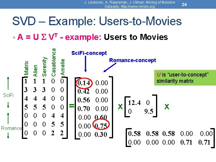
J. Leskovec, A. Rajaraman, J. Ullman: Mining of Massive Datasets, http: //www. mmds. org 24 SVD – Example: Users-to-Movies Serenity Casablanca Amelie Romance Alien Sci. Fi Matrix • A = U VT - example: Users to Movies 1 3 4 5 0 0 0 0 4 5 2 0 0 4 5 2 Sci. Fi-concept Romance-concept = 0. 14 0. 42 0. 56 0. 70 0. 00 0. 60 0. 75 0. 30 U is “user-to-concept” similarity matrix x 12. 4 0 0 9. 5 x 0. 58 0. 00 0. 71

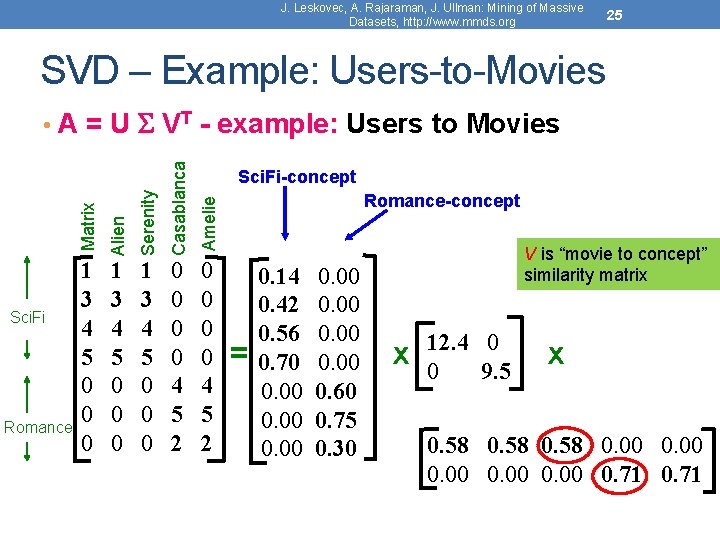
J. Leskovec, A. Rajaraman, J. Ullman: Mining of Massive Datasets, http: //www. mmds. org 25 SVD – Example: Users-to-Movies Serenity Casablanca Amelie Romance Alien Sci. Fi Matrix • A = U VT - example: Users to Movies 1 3 4 5 0 0 0 0 4 5 2 0 0 4 5 2 Sci. Fi-concept Romance-concept = 0. 14 0. 42 0. 56 0. 70 0. 00 0. 60 0. 75 0. 30 V is “movie to concept” similarity matrix x 12. 4 0 0 9. 5 x 0. 58 0. 00 0. 71

J. Leskovec, A. Rajaraman, J. Ullman: Mining of Massive Datasets, http: //www. mmds. org 26 SVD – Example: Users-to-Movies Serenity Casablanca Amelie Romance Alien Sci. Fi Matrix • A = U VT - example: Users to Movies 1 3 4 5 0 0 0 0 4 5 2 0 0 4 5 2 Sci. Fi-concept Romance-concept = 0. 14 0. 42 0. 56 0. 70 0. 00 0. 60 0. 75 0. 30 Σ is the “concept strength” matrix x 12. 4 0 0 9. 5 x 0. 58 0. 00 0. 71

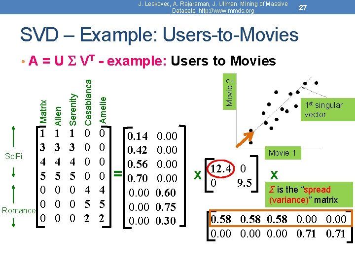
J. Leskovec, A. Rajaraman, J. Ullman: Mining of Massive Datasets, http: //www. mmds. org 27 SVD – Example: Users-to-Movies Casablanca Amelie 1 3 4 5 0 0 0 0 4 5 2 0 0 4 5 2 Movie 2 Serenity Romance Alien Sci. Fi Matrix • A = U VT - example: Users to Movies = 0. 14 0. 42 0. 56 0. 70 0. 00 0. 60 0. 75 0. 30 1 st singular vector Movie 1 x 12. 4 0 0 9. 5 x Σ is the “spread (variance)” matrix 0. 58 0. 00 0. 71

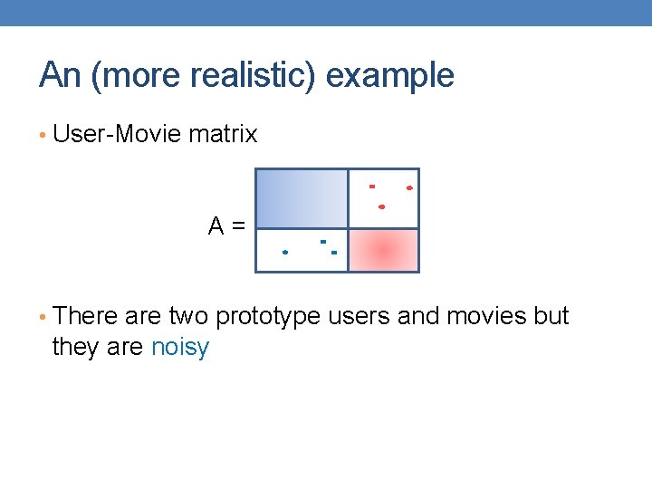
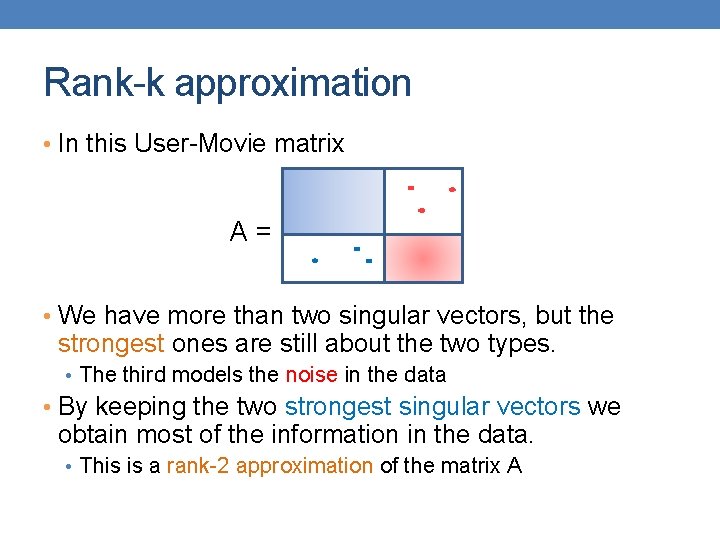
An (more realistic) example • User-Movie matrix A= • There are two prototype users and movies but they are noisy

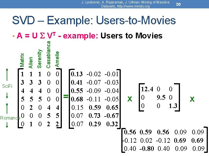
J. Leskovec, A. Rajaraman, J. Ullman: Mining of Massive Datasets, http: //www. mmds. org 29 SVD – Example: Users-to-Movies Matrix Alien Serenity Casablanca Amelie • A = U VT - example: Users to Movies 1 3 Sci. Fi 4 5 0 Romnce 0 0 1 3 4 5 2 0 1 1 3 4 5 0 0 0 0 4 5 2 n = m U VT “Concepts” AKA Latent dimensions AKA Latent factors

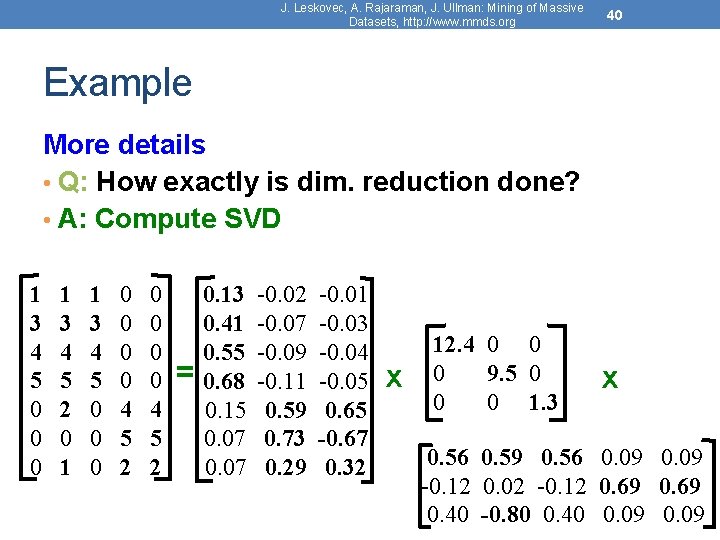
J. Leskovec, A. Rajaraman, J. Ullman: Mining of Massive Datasets, http: //www. mmds. org 30 SVD – Example: Users-to-Movies Matrix Alien Serenity Casablanca Amelie • A = U VT - example: Users to Movies 1 3 Sci. Fi 4 5 0 Romance 0 0 1 3 4 5 2 0 1 1 3 4 5 0 0 0 0 4 5 2 0. 13 0. 41 0. 55 = 0. 68 0. 15 0. 07 -0. 02 -0. 07 -0. 09 -0. 11 0. 59 0. 73 0. 29 -0. 01 -0. 03 -0. 04 -0. 05 0. 65 -0. 67 0. 32 x 12. 4 0 0 0 9. 5 0 0 0 1. 3 x 0. 56 0. 59 0. 56 0. 09 -0. 12 0. 02 -0. 12 0. 69 0. 40 -0. 80 0. 40 0. 09

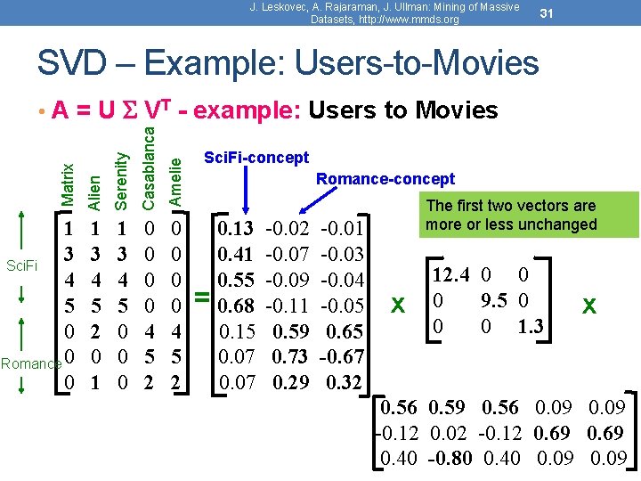
J. Leskovec, A. Rajaraman, J. Ullman: Mining of Massive Datasets, http: //www. mmds. org 31 SVD – Example: Users-to-Movies Matrix Alien Serenity Casablanca Amelie • A = U VT - example: Users to Movies 1 3 Sci. Fi 4 5 0 Romance 0 0 1 3 4 5 2 0 1 1 3 4 5 0 0 0 0 4 5 2 Sci. Fi-concept Romance-concept 0. 13 0. 41 0. 55 = 0. 68 0. 15 0. 07 -0. 02 -0. 07 -0. 09 -0. 11 0. 59 0. 73 0. 29 -0. 01 -0. 03 -0. 04 -0. 05 0. 65 -0. 67 0. 32 The first two vectors are more or less unchanged x 12. 4 0 0 0 9. 5 0 0 0 1. 3 x 0. 56 0. 59 0. 56 0. 09 -0. 12 0. 02 -0. 12 0. 69 0. 40 -0. 80 0. 40 0. 09

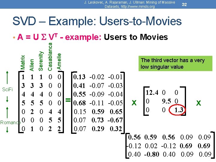
J. Leskovec, A. Rajaraman, J. Ullman: Mining of Massive Datasets, http: //www. mmds. org 32 SVD – Example: Users-to-Movies Matrix Alien Serenity Casablanca Amelie • A = U VT - example: Users to Movies 1 3 Sci. Fi 4 5 0 Romance 0 0 1 3 4 5 2 0 1 1 3 4 5 0 0 0 0 4 5 2 The third vector has a very low singular value 0. 13 0. 41 0. 55 = 0. 68 0. 15 0. 07 -0. 02 -0. 07 -0. 09 -0. 11 0. 59 0. 73 0. 29 -0. 01 -0. 03 -0. 04 -0. 05 0. 65 -0. 67 0. 32 x 12. 4 0 0 0 9. 5 0 0 0 1. 3 x 0. 56 0. 59 0. 56 0. 09 -0. 12 0. 02 -0. 12 0. 69 0. 40 -0. 80 0. 40 0. 09

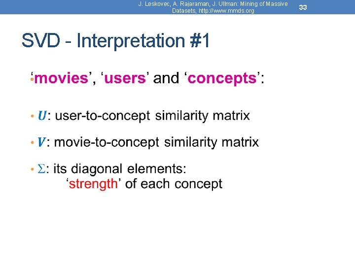
J. Leskovec, A. Rajaraman, J. Ullman: Mining of Massive Datasets, http: //www. mmds. org SVD - Interpretation #1 • 33

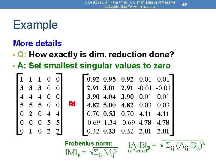
Rank-k approximation • In this User-Movie matrix A= • We have more than two singular vectors, but the strongest ones are still about the two types. • The third models the noise in the data • By keeping the two strongest singular vectors we obtain most of the information in the data. • This is a rank-2 approximation of the matrix A

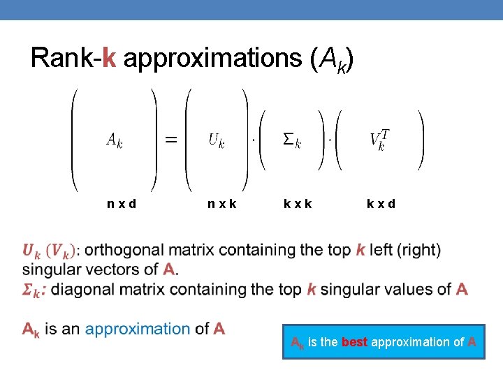
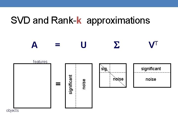
Rank-k approximations (Ak) nxd nxk kxd Ak is the best approximation of A

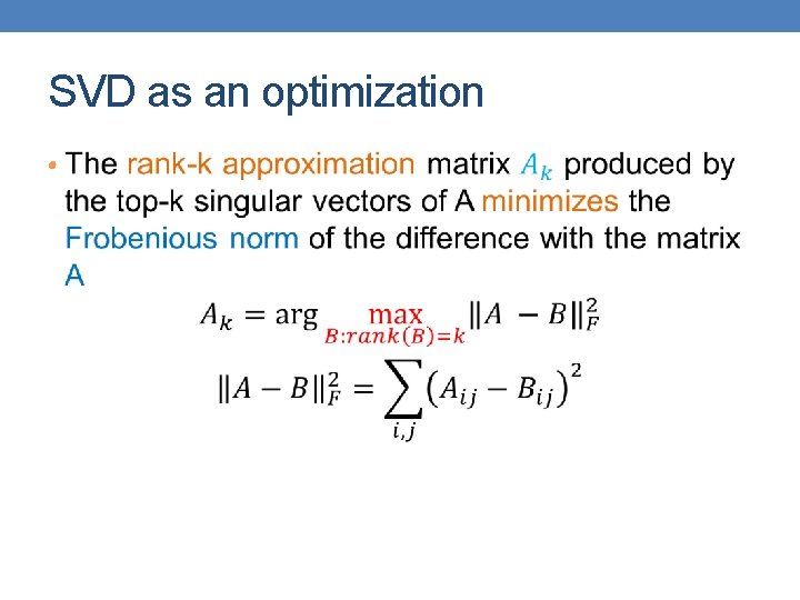
SVD as an optimization •

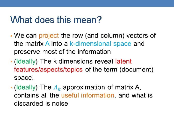
What does this mean? •

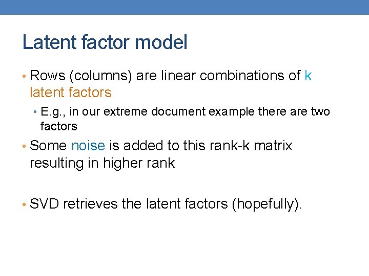
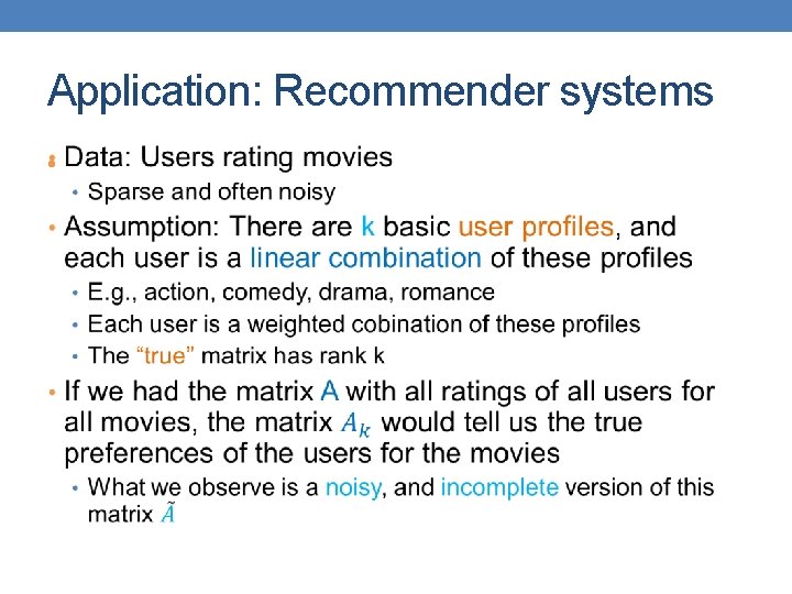
Latent factor model • Rows (columns) are linear combinations of k latent factors • E. g. , in our extreme document example there are two factors • Some noise is added to this rank-k matrix resulting in higher rank • SVD retrieves the latent factors (hopefully).

SVD and Rank-k approximations A = U VT features objects noise = significant noise

J. Leskovec, A. Rajaraman, J. Ullman: Mining of Massive Datasets, http: //www. mmds. org 40 Example More details • Q: How exactly is dim. reduction done? • A: Compute SVD 1 3 4 5 0 0 0 1 3 4 5 2 0 1 1 3 4 5 0 0 0 0 4 5 2 = 0. 13 0. 41 0. 55 0. 68 0. 15 0. 07 -0. 02 -0. 07 -0. 09 -0. 11 0. 59 0. 73 0. 29 -0. 01 -0. 03 -0. 04 -0. 05 0. 65 -0. 67 0. 32 x 12. 4 0 0 0 9. 5 0 0 0 1. 3 x 0. 56 0. 59 0. 56 0. 09 -0. 12 0. 02 -0. 12 0. 69 0. 40 -0. 80 0. 40 0. 09

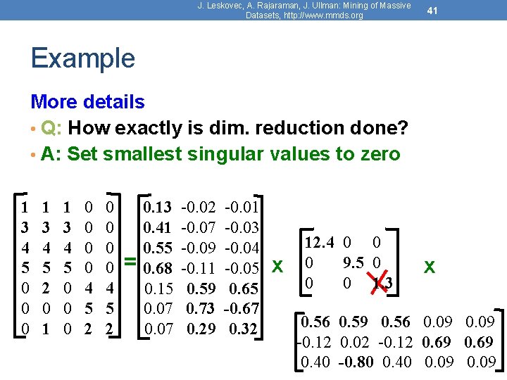
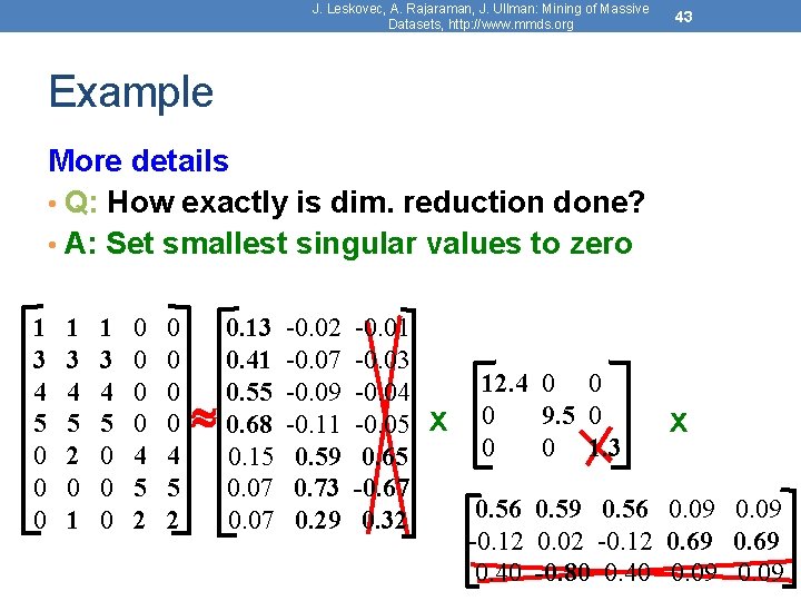
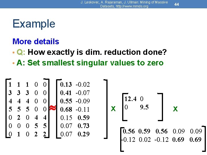
J. Leskovec, A. Rajaraman, J. Ullman: Mining of Massive Datasets, http: //www. mmds. org 41 Example More details • Q: How exactly is dim. reduction done? • A: Set smallest singular values to zero 1 3 4 5 0 0 0 1 3 4 5 2 0 1 1 3 4 5 0 0 0 0 4 5 2 = 0. 13 0. 41 0. 55 0. 68 0. 15 0. 07 -0. 02 -0. 07 -0. 09 -0. 11 0. 59 0. 73 0. 29 -0. 01 -0. 03 -0. 04 -0. 05 0. 65 -0. 67 0. 32 x 12. 4 0 0 0 9. 5 0 0 0 1. 3 x 0. 56 0. 59 0. 56 0. 09 -0. 12 0. 02 -0. 12 0. 69 0. 40 -0. 80 0. 40 0. 09

J. Leskovec, A. Rajaraman, J. Ullman: Mining of Massive Datasets, http: //www. mmds. org 42 Example More details • Q: How exactly is dim. reduction done? • A: Set smallest singular values to zero 1 3 4 5 0 0 0 1 3 4 5 2 0 1 1 3 4 5 0 0 0 0 4 5 2 0. 13 0. 41 0. 55 0. 68 0. 15 0. 07 -0. 02 -0. 07 -0. 09 -0. 11 0. 59 0. 73 0. 29 -0. 01 -0. 03 -0. 04 -0. 05 0. 65 -0. 67 0. 32 x 12. 4 0 0 0 9. 5 0 0 0 1. 3 x 0. 56 0. 59 0. 56 0. 09 -0. 12 0. 02 -0. 12 0. 69 0. 40 -0. 80 0. 40 0. 09

J. Leskovec, A. Rajaraman, J. Ullman: Mining of Massive Datasets, http: //www. mmds. org 43 Example More details • Q: How exactly is dim. reduction done? • A: Set smallest singular values to zero 1 3 4 5 0 0 0 1 3 4 5 2 0 1 1 3 4 5 0 0 0 0 4 5 2 0. 13 0. 41 0. 55 0. 68 0. 15 0. 07 -0. 02 -0. 07 -0. 09 -0. 11 0. 59 0. 73 0. 29 -0. 01 -0. 03 -0. 04 -0. 05 0. 65 -0. 67 0. 32 x 12. 4 0 0 0 9. 5 0 0 0 1. 3 x 0. 56 0. 59 0. 56 0. 09 -0. 12 0. 02 -0. 12 0. 69 0. 40 -0. 80 0. 40 0. 09

J. Leskovec, A. Rajaraman, J. Ullman: Mining of Massive Datasets, http: //www. mmds. org 44 Example More details • Q: How exactly is dim. reduction done? • A: Set smallest singular values to zero 1 3 4 5 0 0 0 1 3 4 5 2 0 1 1 3 4 5 0 0 0 0 4 5 2 0. 13 0. 41 0. 55 0. 68 0. 15 0. 07 -0. 02 -0. 07 -0. 09 -0. 11 0. 59 0. 73 0. 29 x 12. 4 0 0 9. 5 x 0. 56 0. 59 0. 56 0. 09 -0. 12 0. 02 -0. 12 0. 69

J. Leskovec, A. Rajaraman, J. Ullman: Mining of Massive Datasets, http: //www. mmds. org 45 Example More details • Q: How exactly is dim. reduction done? • A: Set smallest singular values to zero 1 3 4 5 0 0 0 1 3 4 5 2 0 1 1 3 4 5 0 0 0 0 4 5 2 0. 92 2. 91 3. 90 4. 82 0. 70 -0. 69 0. 32 0. 95 3. 01 4. 04 5. 00 0. 53 1. 34 0. 23 Frobenius norm: ǁMǁF = Σij Mij 2 0. 92 2. 91 3. 90 4. 82 0. 70 -0. 69 0. 32 0. 01 -0. 01 0. 03 4. 11 4. 78 2. 01 ǁA-BǁF = Σij (Aij-Bij)2 is “small”

Application: Recommender systems •

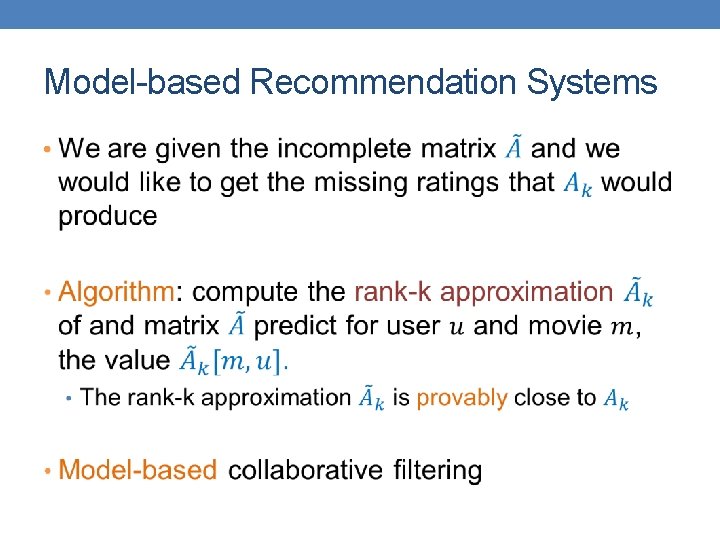
Model-based Recommendation Systems •

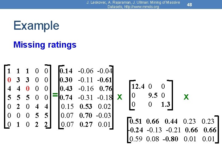
J. Leskovec, A. Rajaraman, J. Ullman: Mining of Massive Datasets, http: //www. mmds. org 48 Example Missing ratings 1 0 4 5 0 0 0 1 3 4 5 2 0 1 1 3 0 5 0 0 0 0 4 5 2 0. 14 0. 30 0. 43 = 0. 74 0. 15 0. 07 -0. 06 -0. 04 -0. 11 -0. 61 -0. 16 0. 76 -0. 31 -0. 18 0. 53 0. 02 0. 70 -0. 03 0. 27 0. 01 x 12. 4 0 0 0 9. 5 0 0 0 1. 3 x 0. 51 0. 66 0. 44 0. 23 -0. 24 -0. 13 -0. 21 0. 66 0. 59 0. 08 -0. 80 0. 01

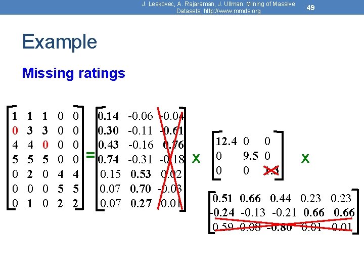
J. Leskovec, A. Rajaraman, J. Ullman: Mining of Massive Datasets, http: //www. mmds. org 49 Example Missing ratings 1 0 4 5 0 0 0 1 3 4 5 2 0 1 1 3 0 5 0 0 0 0 4 5 2 0. 14 0. 30 0. 43 = 0. 74 0. 15 0. 07 -0. 06 -0. 04 -0. 11 -0. 61 -0. 16 0. 76 -0. 31 -0. 18 0. 53 0. 02 0. 70 -0. 03 0. 27 0. 01 x 12. 4 0 0 0 9. 5 0 0 0 1. 3 x 0. 51 0. 66 0. 44 0. 23 -0. 24 -0. 13 -0. 21 0. 66 0. 59 0. 08 -0. 80 0. 01

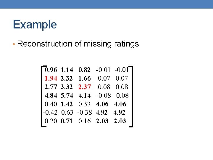
Example • Reconstruction of missing ratings 0. 96 1. 94 2. 77 4. 84 0. 40 -0. 42 0. 20 1. 14 2. 32 3. 32 5. 74 1. 42 0. 63 0. 71 0. 82 1. 66 2. 37 4. 14 0. 33 -0. 38 0. 16 -0. 01 0. 07 0. 08 -0. 08 4. 06 4. 92 2. 03 -0. 01 0. 07 0. 08 4. 06 4. 92 2. 03

SVD and PCA • PCA is a special case of SVD on the centered covariance matrix.

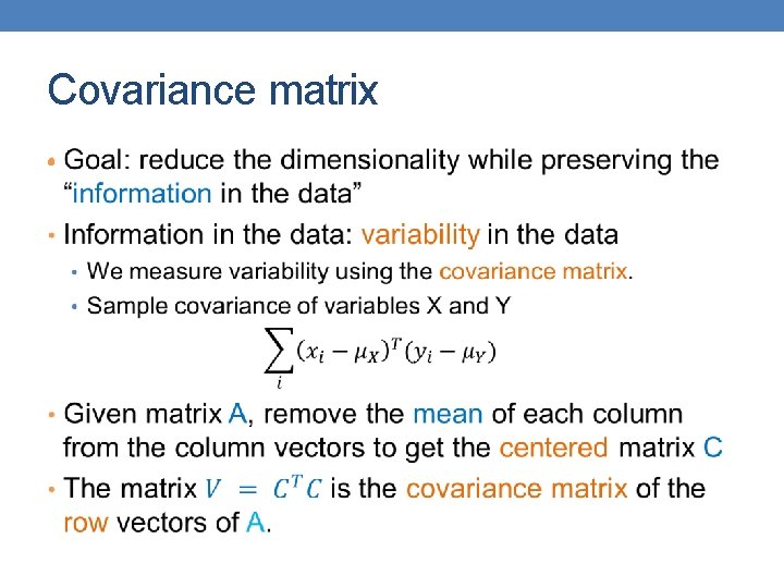
Covariance matrix •

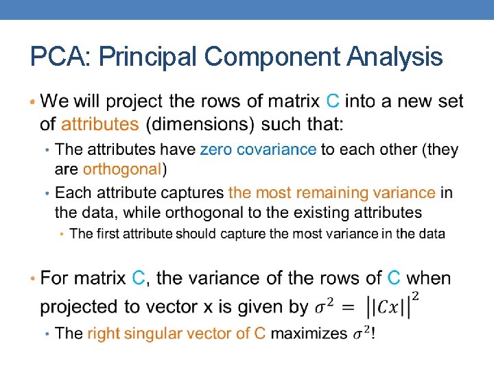
PCA: Principal Component Analysis •

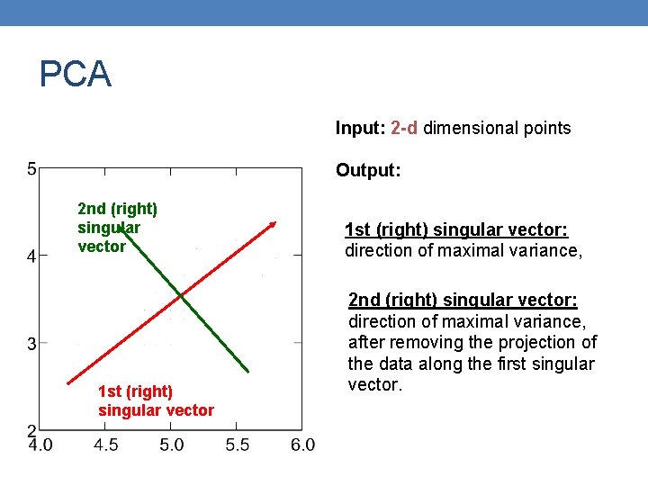
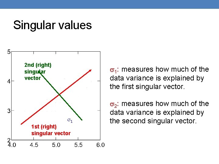
PCA Input: 2 -d dimensional points Output: 2 nd (right) singular vector 1 st (right) singular vector: direction of maximal variance, 2 nd (right) singular vector: direction of maximal variance, after removing the projection of the data along the first singular vector.

Singular values 2 nd (right) singular vector 1: measures how much of the data variance is explained by the first singular vector. 1 1 st (right) singular vector 2: measures how much of the data variance is explained by the second singular vector.

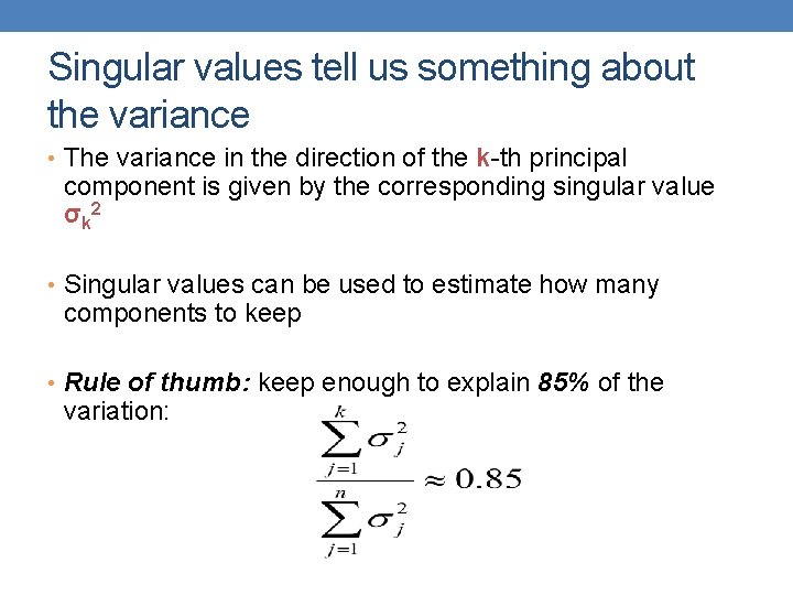
Singular values tell us something about the variance • The variance in the direction of the k-th principal component is given by the corresponding singular value σk 2 • Singular values can be used to estimate how many components to keep • Rule of thumb: keep enough to explain 85% of the variation:

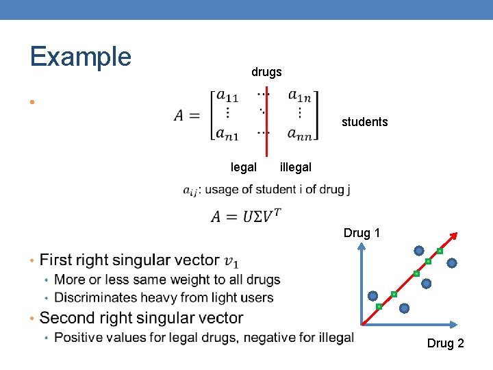
Example drugs • students legal illegal Drug 1 Drug 2

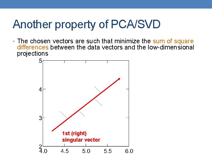
Another property of PCA/SVD • The chosen vectors are such that minimize the sum of square differences between the data vectors and the low-dimensional projections 1 st (right) singular vector

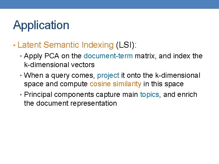
Application • Latent Semantic Indexing (LSI): • Apply PCA on the document-term matrix, and index the k-dimensional vectors • When a query comes, project it onto the k-dimensional space and compute cosine similarity in this space • Principal components capture main topics, and enrich the document representation

SVD is “the Rolls-Royce and the Swiss Army Knife of Numerical Linear Algebra. ”* *Dianne O’Leary, MMDS ’ 06

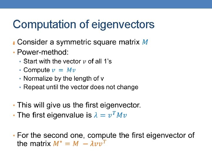
Computation of eigenvectors •

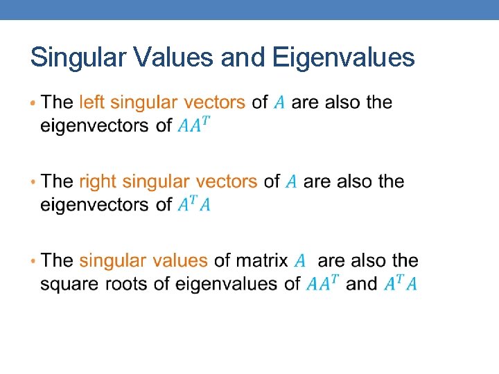
Singular Values and Eigenvalues •

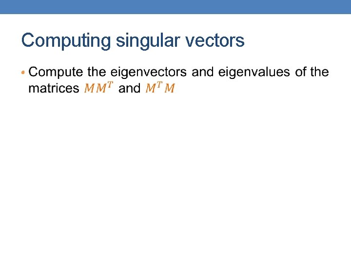
Computing singular vectors •