Dimensionality reduction PCA MDS ISOMAP SVD ICA s

Dimensionality reduction PCA, MDS, ISOMAP, SVD, ICA, s. PCA CSCE 883

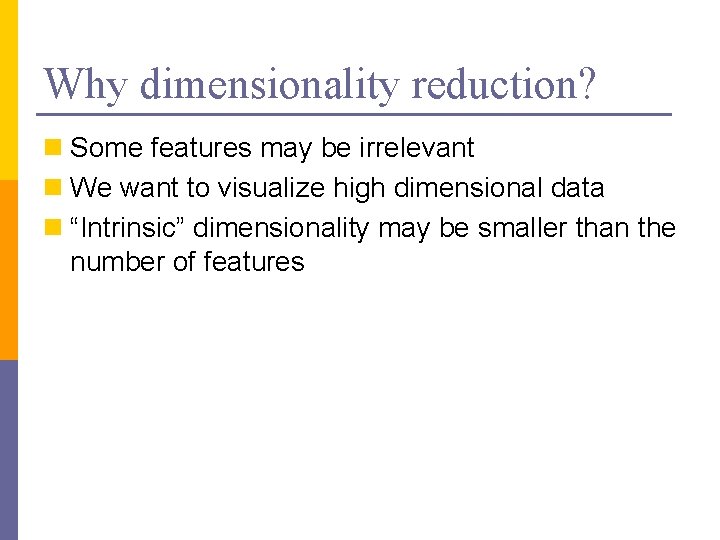
Why dimensionality reduction? n Some features may be irrelevant n We want to visualize high dimensional data n “Intrinsic” dimensionality may be smaller than the number of features

Global Mapping of Protein Structure Space

Isomap on face images 4

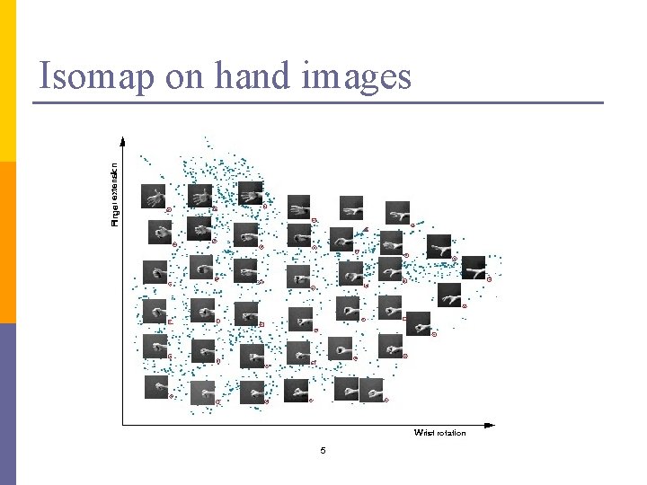
Isomap on hand images 5

Isomap on written two-s 6

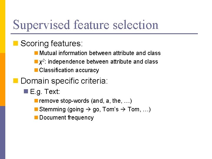
Supervised feature selection n Scoring features: n Mutual information between attribute and class n χ2: independence between attribute and class n Classification accuracy n Domain specific criteria: n E. g. Text: n remove stop-words (and, a, the, …) n Stemming (going go, Tom’s Tom, …) n Document frequency

Choosing sets of features n Score each feature n Forward/Backward elimination n Choose the feature with the highest/lowest score n Re-score other features n Repeat n If you have lots of features (like in text) n Just select top K scored features

Feature selection on text SVM k. NN Rochio NB

Unsupervised feature selection n Differs from feature selection in two ways: n Instead of choosing subset of features, n Create new features (dimensions) defined as functions over all features n Don’t consider class labels, just the data points

Unsupervised feature selection n Idea: n Given data points in d-dimensional space, n Project into lower dimensional space while preserving as much information as possible n E. g. , find best planar approximation to 3 D data n E. g. , find best planar approximation to 104 D data n In particular, choose projection that minimizes the squared error in reconstructing original data

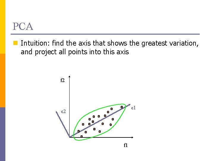
PCA n Intuition: find the axis that shows the greatest variation, and project all points into this axis f 2 e 1 e 2 f 1

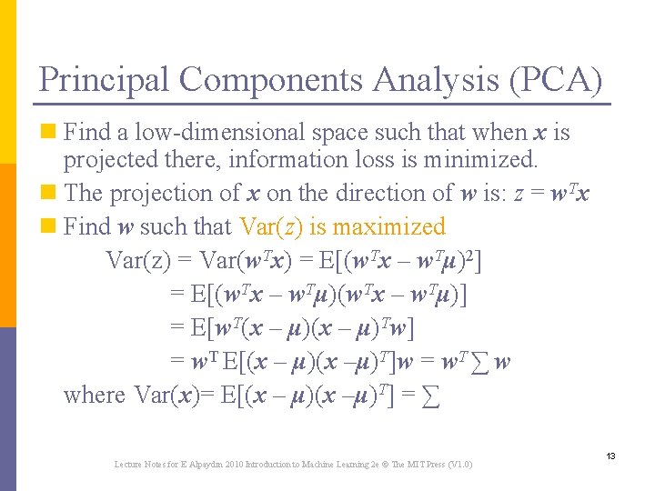
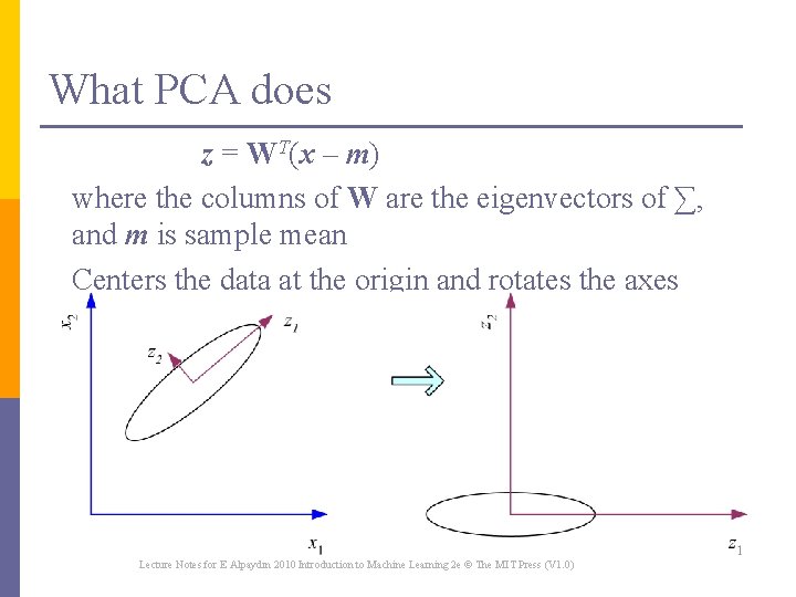
Principal Components Analysis (PCA) n Find a low-dimensional space such that when x is projected there, information loss is minimized. n The projection of x on the direction of w is: z = w. Tx n Find w such that Var(z) is maximized Var(z) = Var(w. Tx) = E[(w. Tx – w. Tμ)2] = E[(w. Tx – w. Tμ)] = E[w. T(x – μ)Tw] = w. T E[(x – μ)(x –μ)T]w = w. T ∑ w where Var(x)= E[(x – μ)(x –μ)T] = ∑ Lecture Notes for E Alpaydın 2010 Introduction to Machine Learning 2 e © The MIT Press (V 1. 0) 13

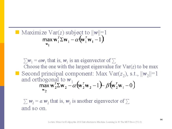
n Maximize Var(z) subject to ||w||=1 ∑w 1 = αw 1 that is, w 1 is an eigenvector of ∑ Choose the one with the largest eigenvalue for Var(z) to be max n Second principal component: Max Var(z 2), s. t. , ||w 2||=1 and orthogonal to w 1 ∑ w 2 = α w 2 that is, w 2 is another eigenvector of ∑ and so on. Lecture Notes for E Alpaydın 2010 Introduction to Machine Learning 2 e © The MIT Press (V 1. 0) 14

What PCA does z = WT(x – m) where the columns of W are the eigenvectors of ∑, and m is sample mean Centers the data at the origin and rotates the axes Lecture Notes for E Alpaydın 2010 Introduction to Machine Learning 2 e © The MIT Press (V 1. 0) 15

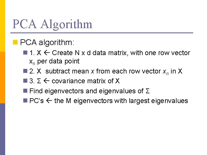
PCA Algorithm n PCA algorithm: n 1. X Create N x d data matrix, with one row vector xn per data point n 2. X subtract mean x from each row vector xn in X n 3. Σ covariance matrix of X n Find eigenvectors and eigenvalues of Σ n PC’s the M eigenvectors with largest eigenvalues

PCA Algorithm in Matlab % generate data Data = mvnrnd([5, 5], [1 1. 5; 1. 5 3], 100); figure(1); plot(Data(: , 1), Data(: , 2), '+'); %center the data for i = 1: size(Data, 1) Data(i, : ) = Data(i, : ) - mean(Data); end Data. Cov = cov(Data); %covariance matrix [PC, variances, explained] = pcacov(Data. Cov); %eigen % plot principal components figure(2); clf; hold on; plot(Data(: , 1), Data(: , 2), '+b'); plot(PC(1, 1)*[-5 5], PC(2, 1)*[-5 5], '-r’) plot(PC(1, 2)*[-5 5], PC(2, 2)*[-5 5], '-b’); hold off % project down to 1 dimension Pca. Pos = Data * PC(: , 1);

2 d Data

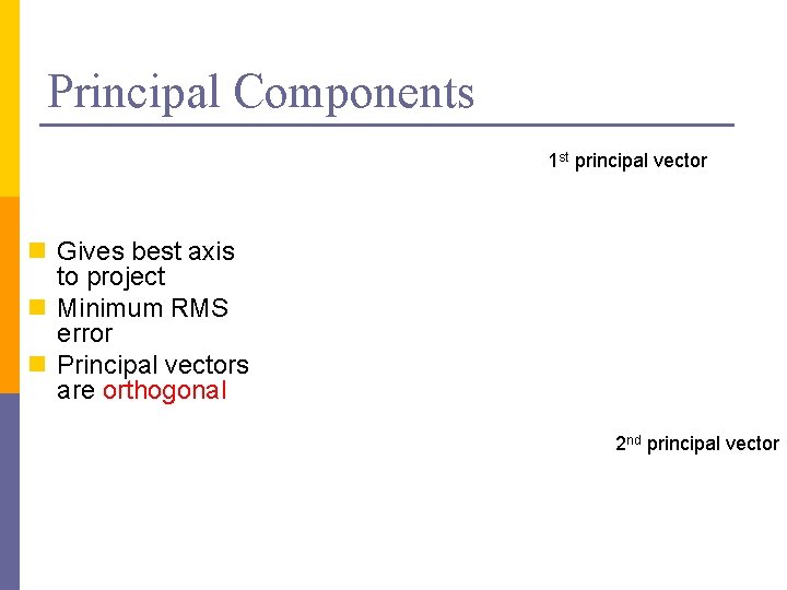
Principal Components 1 st principal vector n Gives best axis to project n Minimum RMS error n Principal vectors are orthogonal 2 nd principal vector

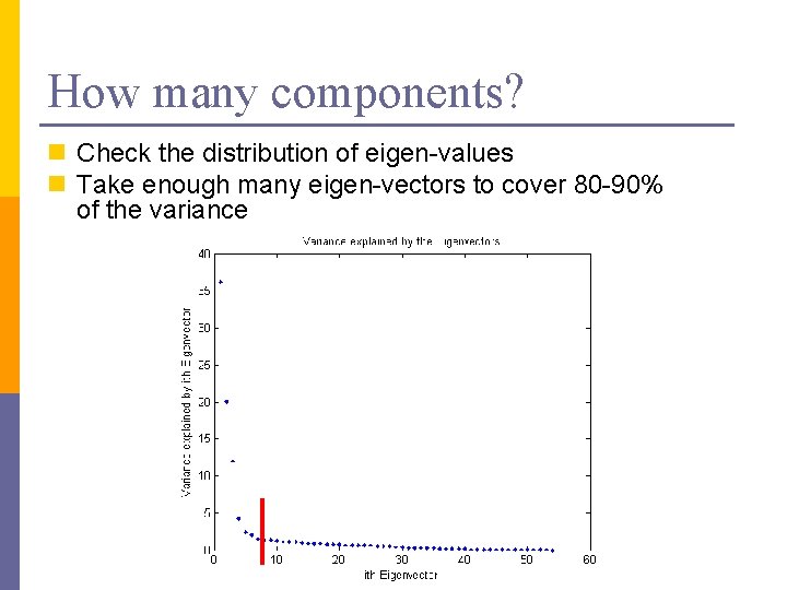
How many components? n Check the distribution of eigen-values n Take enough many eigen-vectors to cover 80 -90% of the variance

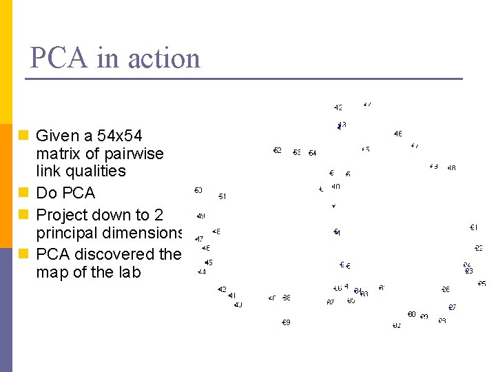
Sensor networks Sensors in Intel Berkeley Lab

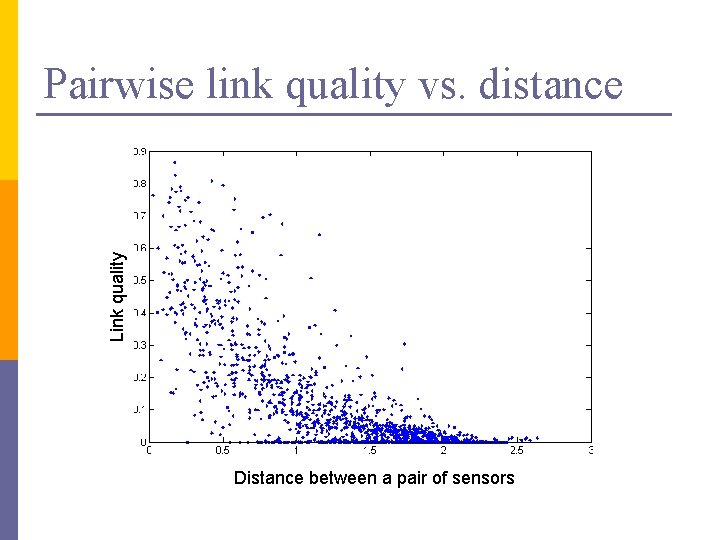
Link quality Pairwise link quality vs. distance Distance between a pair of sensors

PCA in action n Given a 54 x 54 matrix of pairwise link qualities n Do PCA n Project down to 2 principal dimensions n PCA discovered the map of the lab

Problems and limitations n What if very large dimensional data? n e. g. , Images (d ≥ 104) n Problem: n Covariance matrix Σ is size (d 2) n d=104 |Σ| = 108 n Singular Value Decomposition (SVD)! n efficient algorithms available (Matlab) n some implementations find just top N eigenvectors

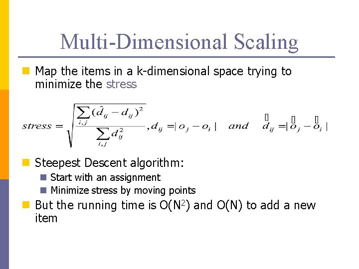
Multi-Dimensional Scaling n Map the items in a k-dimensional space trying to minimize the stress n Steepest Descent algorithm: n Start with an assignment n Minimize stress by moving points n But the running time is O(N 2) and O(N) to add a new item

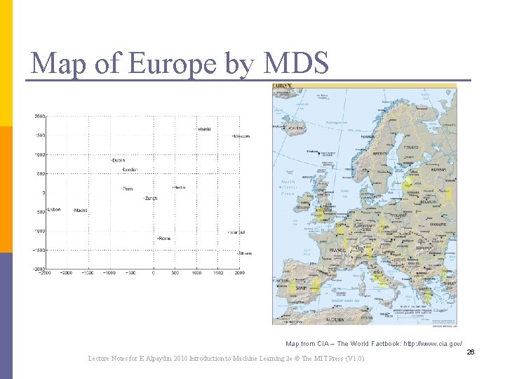
Map of Europe by MDS Map from CIA – The World Factbook: http: //www. cia. gov/ Lecture Notes for E Alpaydın 2010 Introduction to Machine Learning 2 e © The MIT Press (V 1. 0) 26

Global or Topology preserving n Mostly used for visualization and classification n PCA or KL decomposition n MDS n SVD n ICA 27

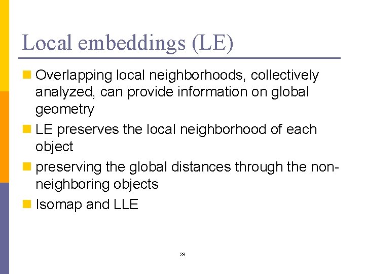
Local embeddings (LE) n Overlapping local neighborhoods, collectively analyzed, can provide information on global geometry n LE preserves the local neighborhood of each object n preserving the global distances through the nonneighboring objects n Isomap and LLE 28

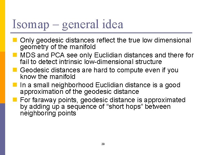
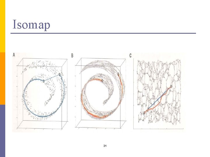
Isomap – general idea n Only geodesic distances reflect the true low dimensional geometry of the manifold n MDS and PCA see only Euclidian distances and there for fail to detect intrinsic low-dimensional structure n Geodesic distances are hard to compute even if you know the manifold n In a small neighborhood Euclidian distance is a good approximation of the geodesic distance n For faraway points, geodesic distance is approximated by adding up a sequence of “short hops” between neighboring points 29

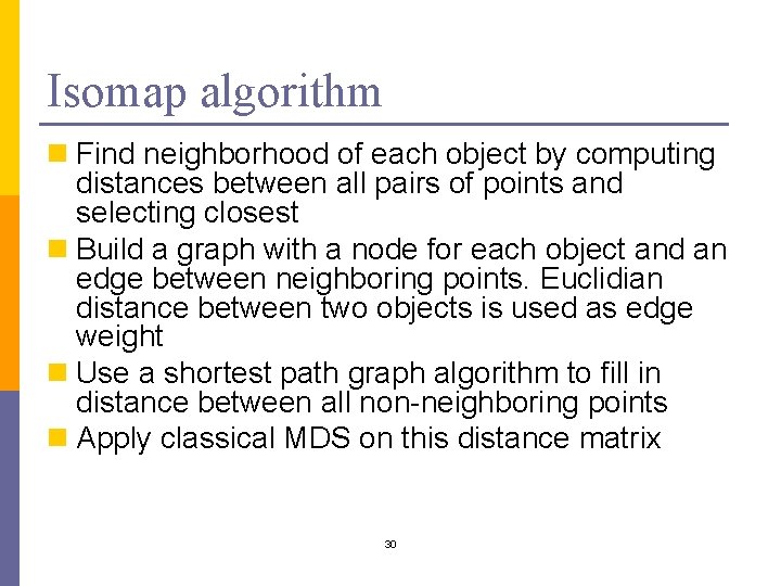
Isomap algorithm n Find neighborhood of each object by computing distances between all pairs of points and selecting closest n Build a graph with a node for each object and an edge between neighboring points. Euclidian distance between two objects is used as edge weight n Use a shortest path graph algorithm to fill in distance between all non-neighboring points n Apply classical MDS on this distance matrix 30

Isomap 31

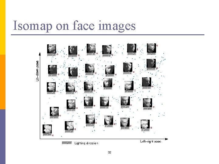
Isomap on face images 32

Isomap on hand images 33

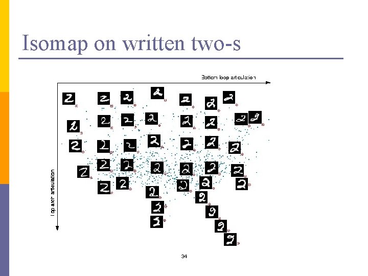
Isomap on written two-s 34

Matlab source from http: //web. mit. edu/cocosci/isomap. html Lecture Notes for E Alpaydın 2010 Introduction to Machine Learning 2 e © The MIT Press (V 1. 0) 35

Isomap - summary n Inherits features of MDS and PCA: n n guaranteed asymptotic convergence to true structure Polynomial runtime Non-iterative Ability to discover manifolds of arbitrary dimensionality n Perform well when data is from a single well sampled cluster n Few free parameters n Good theoretical base for its metrics preserving properties 36

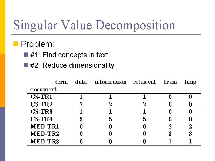
Singular Value Decomposition n Problem: n #1: Find concepts in text n #2: Reduce dimensionality

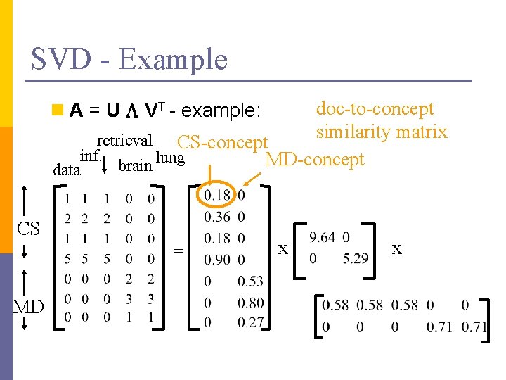
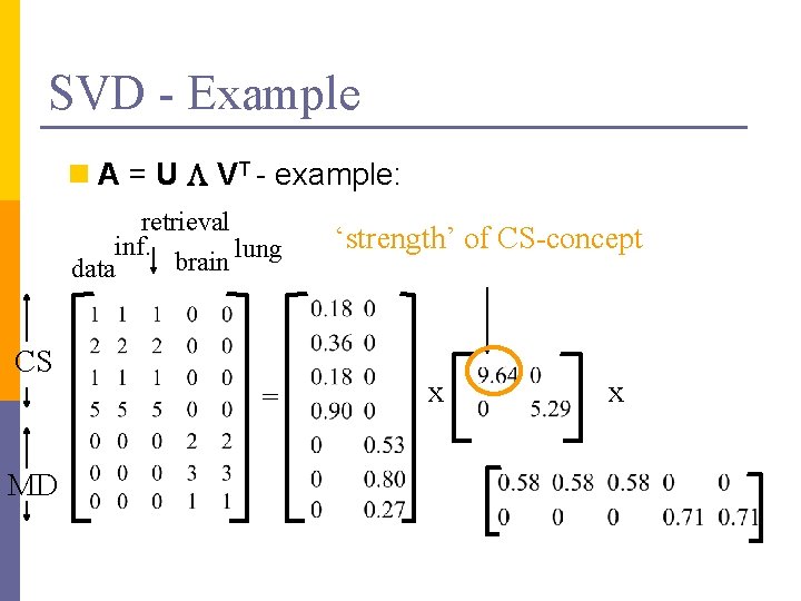
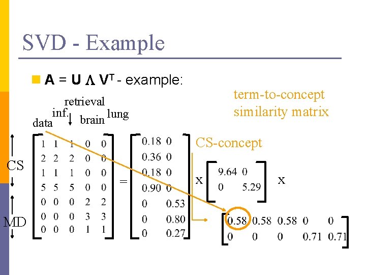
SVD - Definition A[n x m] = U[n x r] L [ r x r] (V[m x r])T n A: n x m matrix (e. g. , n documents, m terms) n U: n x r matrix (n documents, r concepts) n L: r x r diagonal matrix (strength of each ‘concept’) (r: rank of the matrix) n V: m x r matrix (m terms, r concepts)

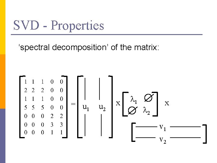
SVD - Properties THEOREM [Press+92]: always possible to decompose matrix A into A = U L VT , where n U, L, V: unique (*) n U, V: column orthonormal (ie. , columns are unit vectors, orthogonal to each other) n UTU = I; VTV = I (I: identity matrix) n L: singular value are positive, and sorted in decreasing order

SVD - Properties ‘spectral decomposition’ of the matrix: = u 1 u 2 x l 1 l 2 x v 1 v 2

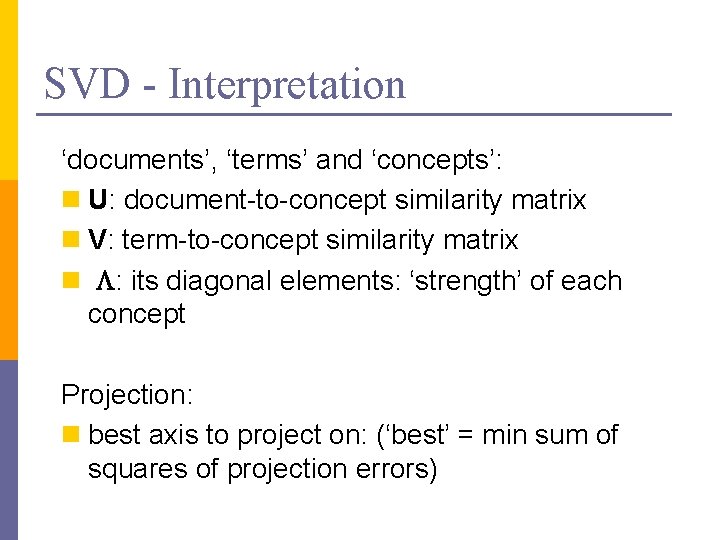
SVD - Interpretation ‘documents’, ‘terms’ and ‘concepts’: n U: document-to-concept similarity matrix n V: term-to-concept similarity matrix n L: its diagonal elements: ‘strength’ of each concept Projection: n best axis to project on: (‘best’ = min sum of squares of projection errors)

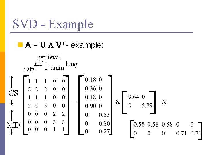
SVD - Example n A = U L VT - example: retrieval inf. lung brain data CS = MD x x

SVD - Example doc-to-concept similarity matrix retrieval CS-concept inf. MD-concept brain lung n A = U L VT - example: data CS = MD x x

SVD - Example n A = U L VT - example: retrieval inf. lung brain data CS = MD ‘strength’ of CS-concept x x

SVD - Example n A = U L VT - example: term-to-concept similarity matrix retrieval inf. lung brain data CS-concept CS = MD x x

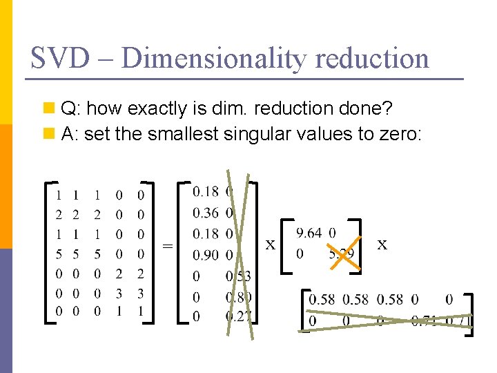
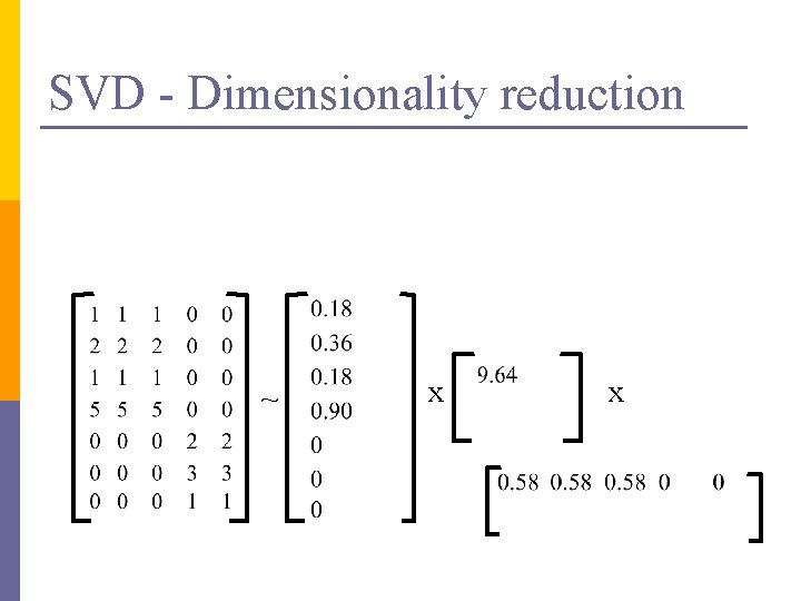
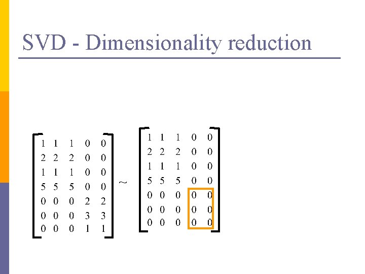
SVD – Dimensionality reduction n Q: how exactly is dim. reduction done? n A: set the smallest singular values to zero: = x x

SVD - Dimensionality reduction ~ x x

SVD - Dimensionality reduction ~

Matlab source from http: //web. mit. edu/cocosci/isomap. html Lecture Notes for E Alpaydın 2010 Introduction to Machine Learning 2 e © The MIT Press (V 1. 0) 50