LSI SVD and Data Management SVD Detailed outline

LSI, SVD and Data Management

SVD - Detailed outline n n n Motivation Definition - properties Interpretation Complexity Case studies Additional properties

SVD - Motivation n n problem #1: text - LSI: find ‘concepts’ problem #2: compression / dim. reduction

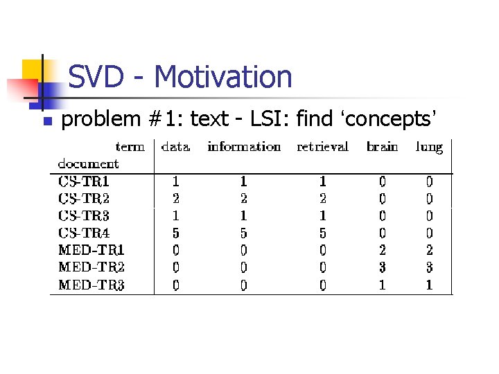
SVD - Motivation n problem #1: text - LSI: find ‘concepts’

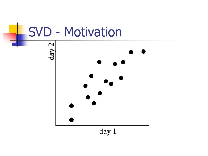
SVD - Motivation n problem #2: compress / reduce dimensionality

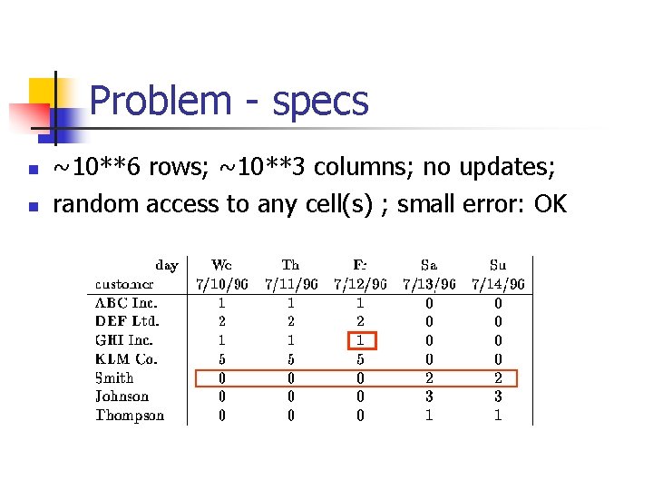
Problem - specs n n ~10**6 rows; ~10**3 columns; no updates; random access to any cell(s) ; small error: OK

SVD - Motivation

SVD - Motivation

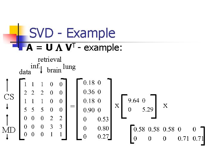
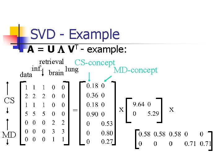
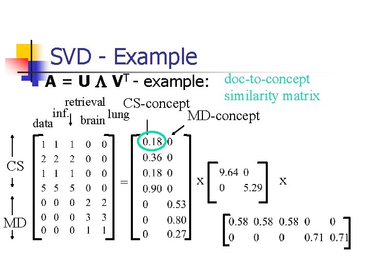
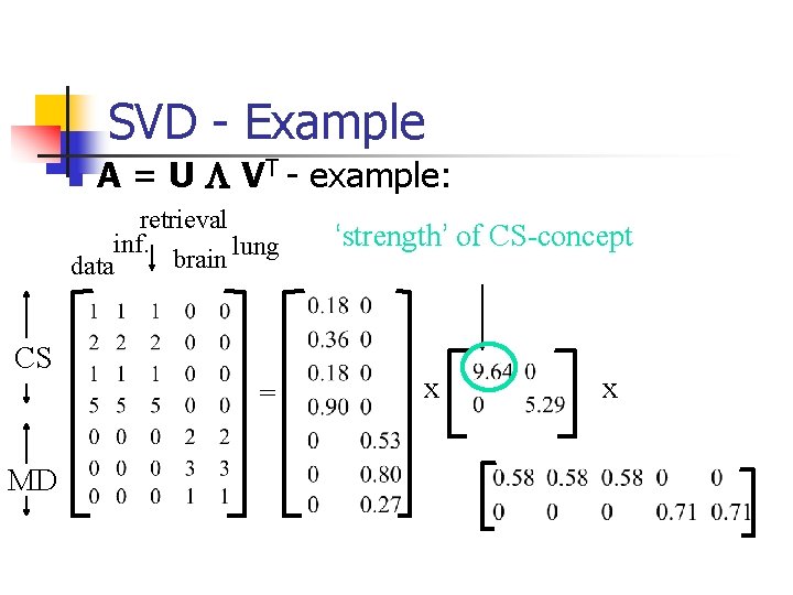
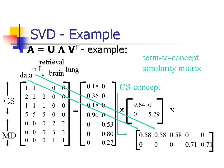
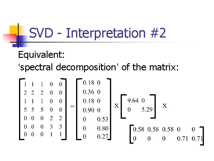
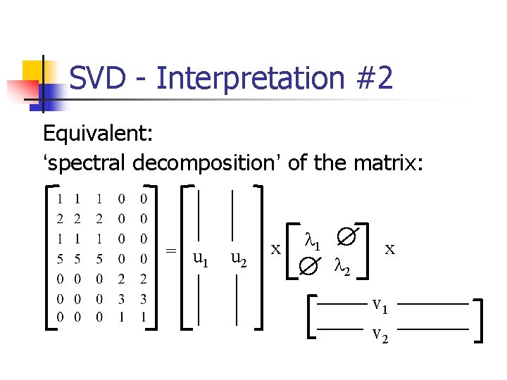
SVD - Definition A[n x m] = U[n x r] L [ r x r] (V[m x r])T n n A: n x m matrix (eg. , n documents, m terms) U: n x r matrix (n documents, r concepts) L: r x r diagonal matrix (strength of each ‘concept’) (r : rank of the matrix) V: m x r matrix (m terms, r concepts)

SVD - Properties THEOREM [Press+92]: always possible to decompose matrix A into A = U L VT , where n U, L, V: unique (*) n U, V: column orthonormal (ie. , columns are unit vectors, orthogonal to each other) n n UT U = I; VT V = I (I: identity matrix) L: singular values, non-negative and sorted in decreasing order

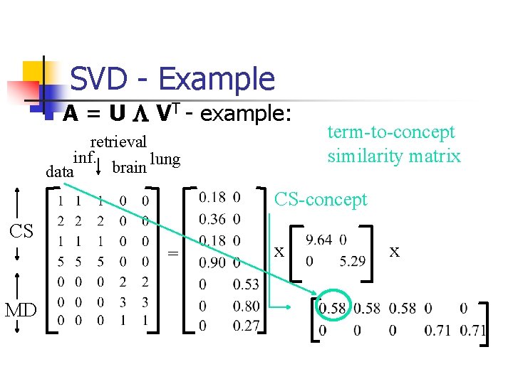
SVD - Example n A = U L VT - example: retrieval inf. lung brain data CS = MD x x

SVD - Example n A = U L VT - example: retrieval CS-concept inf. lung MD-concept brain data CS = MD x x

SVD - Example n A = U L VT - example: doc-to-concept similarity matrix retrieval CS-concept inf. lung MD-concept brain data CS = MD x x

SVD - Example n A = U L VT - example: retrieval inf. lung brain data CS = MD ‘strength’ of CS-concept x x

SVD - Example n A = U L VT - example: retrieval inf. lung brain data term-to-concept similarity matrix CS-concept CS = MD x x

SVD - Example n A = U L VT - example: retrieval inf. lung brain data term-to-concept similarity matrix CS-concept CS = MD x x

SVD - Detailed outline n n n Motivation Definition - properties Interpretation Complexity Case studies Additional properties

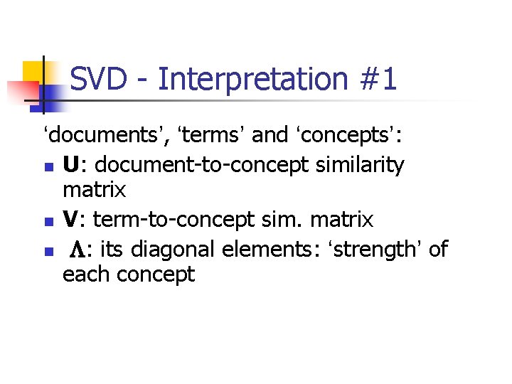
SVD - Interpretation #1 ‘documents’, ‘terms’ and ‘concepts’: n U: document-to-concept similarity matrix n V: term-to-concept sim. matrix n L: its diagonal elements: ‘strength’ of each concept

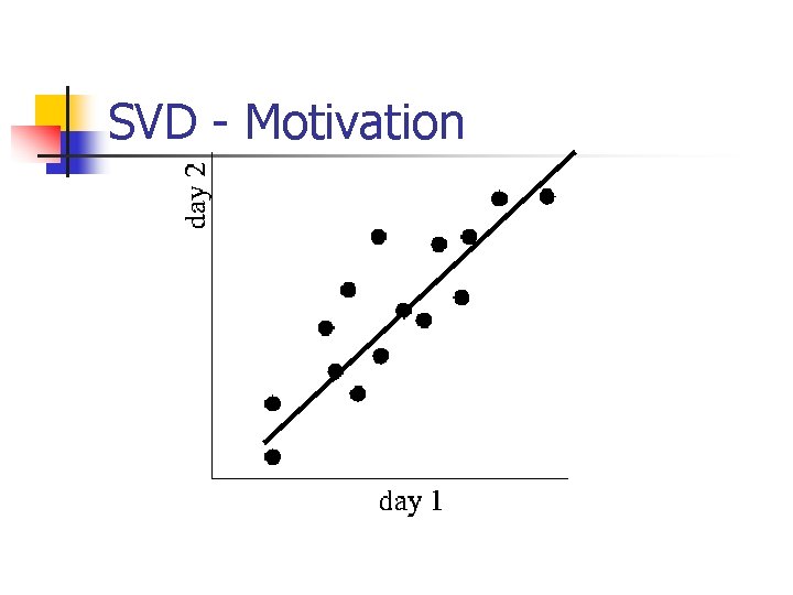
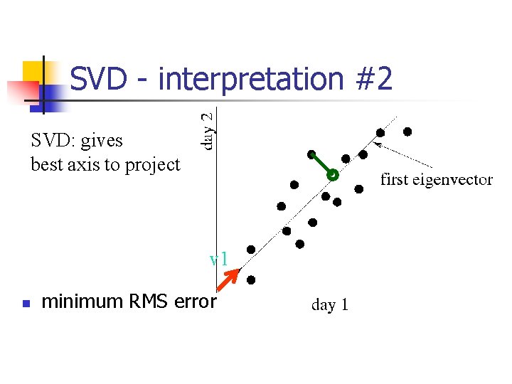
SVD - Interpretation #2 n best axis to project on: (‘best’ = min sum of squares of projection errors)

SVD - Motivation

SVD - interpretation #2 SVD: gives best axis to project v 1 n minimum RMS error

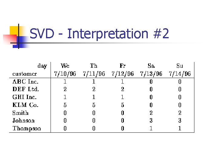
SVD - Interpretation #2

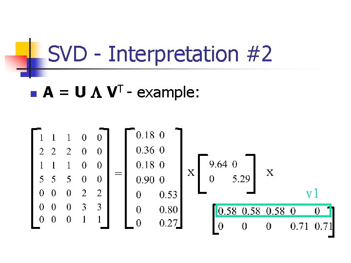
SVD - Interpretation #2 n A = U L VT - example: = x x v 1

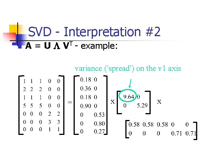
SVD - Interpretation #2 n A = U L VT - example: variance (‘spread’) on the v 1 axis = x x

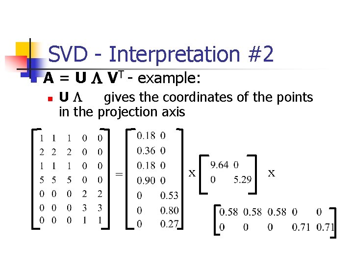
SVD - Interpretation #2 n A = U L VT - example: n UL gives the coordinates of the points in the projection axis = x x

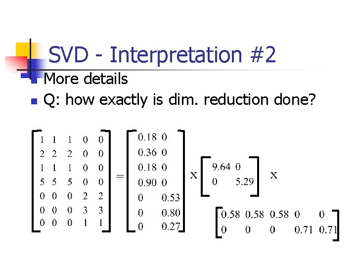
SVD - Interpretation #2 n n More details Q: how exactly is dim. reduction done? = x x

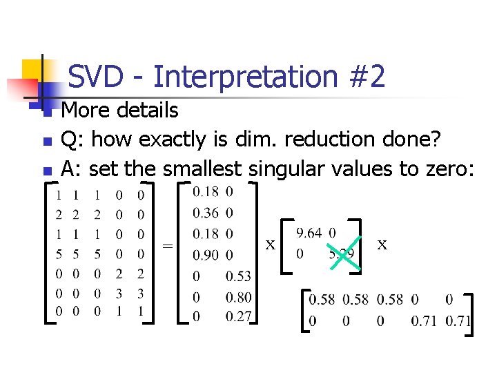
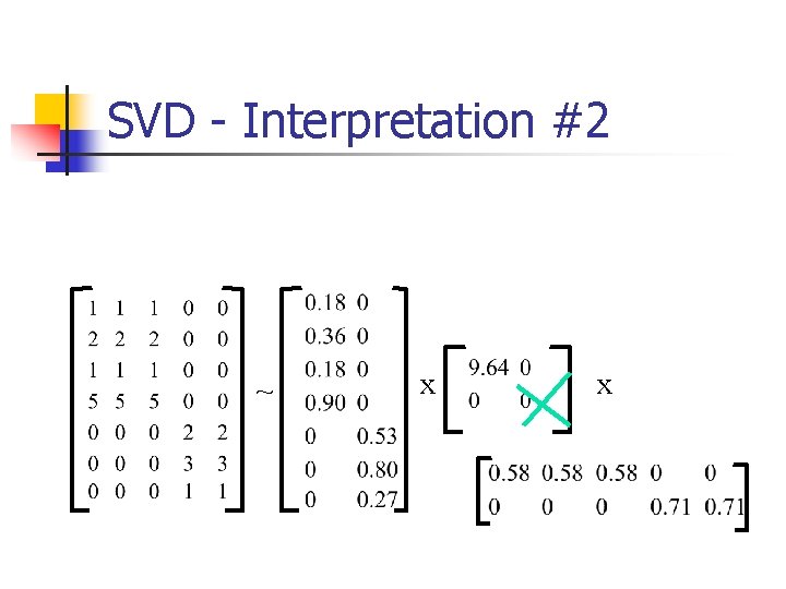
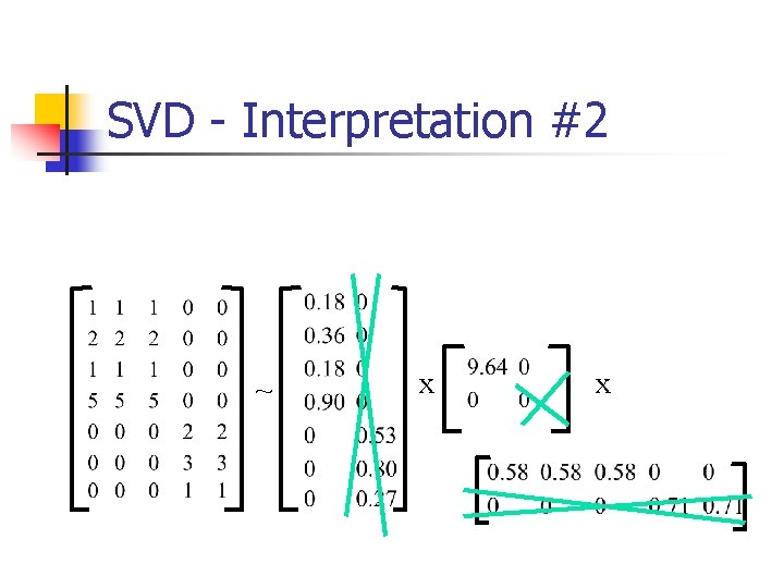
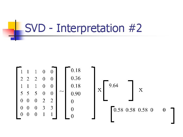
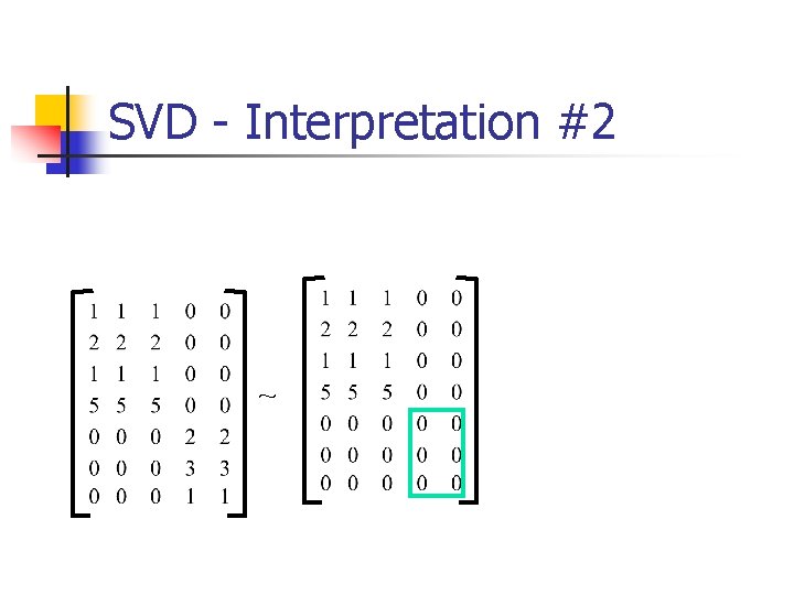
SVD - Interpretation #2 n n n More details Q: how exactly is dim. reduction done? A: set the smallest singular values to zero: = x x

SVD - Interpretation #2 ~ x x

SVD - Interpretation #2 ~ x x

SVD - Interpretation #2 ~ x x

SVD - Interpretation #2 ~

SVD - Interpretation #2 Equivalent: ‘spectral decomposition’ of the matrix: = x x

SVD - Interpretation #2 Equivalent: ‘spectral decomposition’ of the matrix: = u 1 u 2 x l 1 l 2 x v 1 v 2

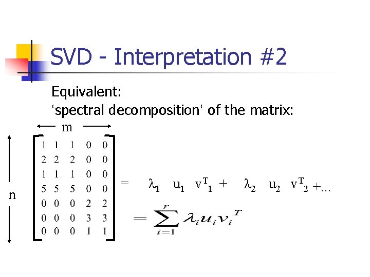
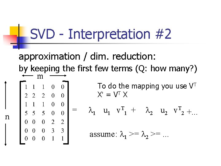
SVD - Interpretation #2 Equivalent: ‘spectral decomposition’ of the matrix: m n = l 1 u 1 v. T 1 + l 2 u 2 v. T 2 +. . .

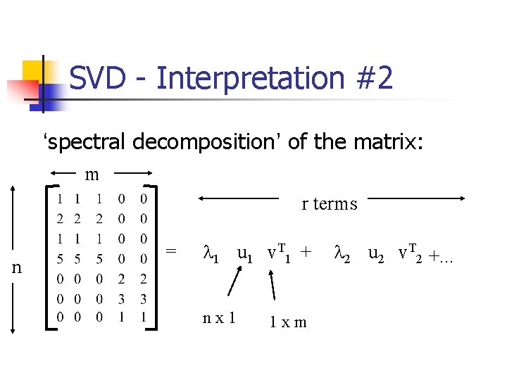
SVD - Interpretation #2 ‘spectral decomposition’ of the matrix: m r terms n = l 1 u 1 v. T 1 + nx 1 1 xm l 2 u 2 v. T 2 +. . .

SVD - Interpretation #2 approximation / dim. reduction: by keeping the first few terms (Q: how many? ) m To do the mapping you use VT X’ = VT X n = l 1 u 1 v. T 1 + l 2 u 2 v. T 2 +. . . assume: l 1 >= l 2 >=. . .

SVD - Interpretation #2 A (heuristic - [Fukunaga]): keep 80 -90% of ‘energy’ (= sum of squares of li ’s) m n = l 1 u 1 v. T 1 + l 2 u 2 v. T 2 +. . . assume: l 1 >= l 2 >=. . .

LSI A[n x m] = U[n x r] L [ r x r] (V[m x r])T then map to A[n x m] = U[n x k] L [ k x k] (V[m x k])T k concepts are the k strongest singular vectors A matrix has rank k

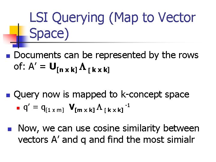
LSI Querying (Map to Vector Space) n n Documents can be represented by the rows of: A’ = U[n x k] L [ k x k] Query now is mapped to k-concept space n n q’ = q[1 x m] V[m x k] L [ k x k] -1 Now, we can use cosine similarity between vectors A’ and q and find the most simialr

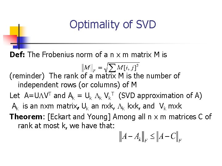
Optimality of SVD Def: The Frobenius norm of a n x m matrix M is (reminder) The rank of a matrix M is the number of independent rows (or columns) of M Let A=ULVT and Ak = Uk Lk Vk. T (SVD approximation of A) Ak is an nxm matrix, Uk an nxk, Lk kxk, and Vk mxk Theorem: [Eckart and Young] Among all n x m matrices C of rank at most k, we have that:

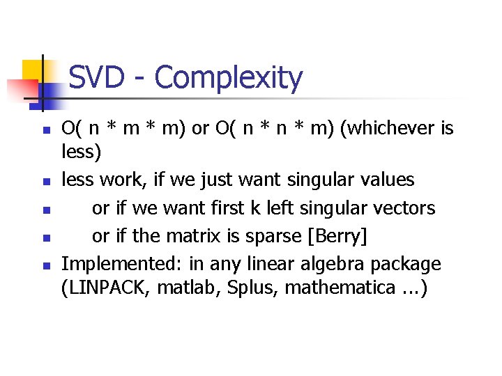
SVD - Complexity n n n O( n * m) or O( n * m) (whichever is less) less work, if we just want singular values or if we want first k left singular vectors or if the matrix is sparse [Berry] Implemented: in any linear algebra package (LINPACK, matlab, Splus, mathematica. . . )

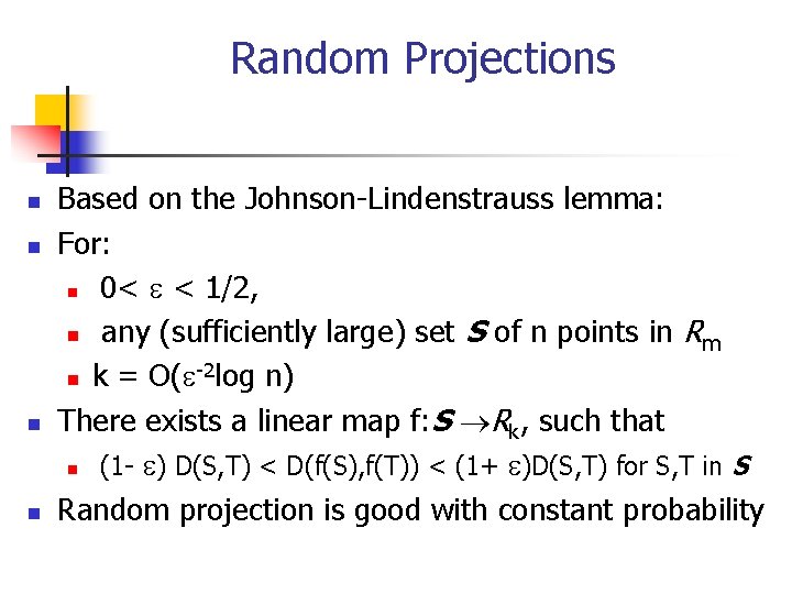
Random Projections n n Based on the Johnson-Lindenstrauss lemma: For: n 0< e < 1/2, n any (sufficiently large) set S of n points in R m -2 n k = O(e log n) There exists a linear map f: S Rk, such that n (1 - e) D(S, T) < D(f(S), f(T)) < (1+ e)D(S, T) for S, T in S Random projection is good with constant probability

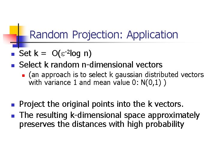
Random Projection: Application n n Set k = O(e-2 log n) Select k random n-dimensional vectors n n n (an approach is to select k gaussian distributed vectors with variance 1 and mean value 0: N(0, 1) ) Project the original points into the k vectors. The resulting k-dimensional space approximately preserves the distances with high probability

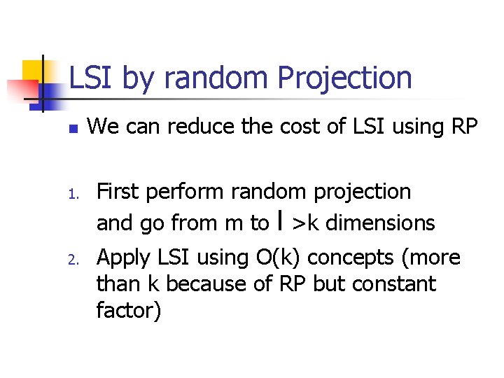
LSI by random Projection n 1. 2. We can reduce the cost of LSI using RP First perform random projection and go from m to l >k dimensions Apply LSI using O(k) concepts (more than k because of RP but constant factor)

LSI: Theory Theoretical justification [Papadimitriou et al. ‘ 98] n If the database consists of k topics, each topic represented by a set of terms, each document comes from one topic by sampling the terms associated with the topic, and topics and documents are well separated n n then LSI works with high probability! Random Projections and then LSI using the correct number of dimensions for each step, is equivalent to LSI! Christos H. Papadimitriou, Prabhakar Raghavan, Hisao Tamaki, Santosh Vempala: Latent Semantic Indexing: A Probabilistic Analysis. PODS 1998: 159 -168