Computational Genomics Lecture 10 Hidden Markov Models HMMs

Computational Genomics Lecture 10 Hidden Markov Models (HMMs) © Ydo Wexler & Dan Geiger (Technion) and by Nir Friedman (HU). Modified by Benny Chor (TAU)

Outline u u u Finite, or Discrete, Markov Models Hidden Markov Models Three major questions: Q 1. : Computing the probability of a given observation. A 1. : Forward – Backward (Baum Welch) dynamic programming algorithm. Q 2. : Computing the most probable sequence, given an observation. A 2. : Viterbi’s dynamic programming Algorithm Q 3. : Learn best model, given an observation, . A 3. : Expectation Maximization (EM): A Heuristic. 2

Markov Models A discrete (finite) system: l N distinct states. l Begins (at time t=1) in some initial state(s). l At each time step (t=1, 2, …) the system moves from current to next state (possibly the same as the current state) according to transition probabilities associated with current state. u This kind of system is called a finite, or discrete Markov model u u After Andrei Andreyevich Markov (1856 -1922) 3

Outline Markov Chains (Markov Models) u Hidden Markov Chains (HMMs) u Algorithmic Questions u Biological Relevance u 4

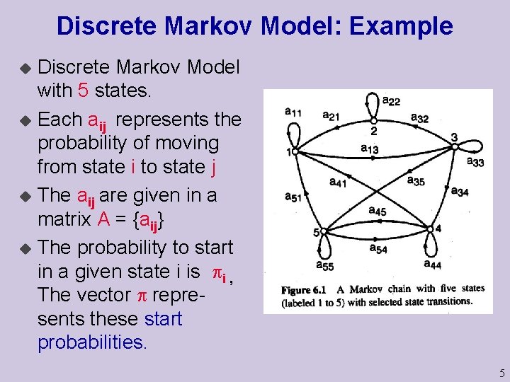
Discrete Markov Model: Example Discrete Markov Model with 5 states. u Each aij represents the probability of moving from state i to state j u The aij are given in a matrix A = {aij} u The probability to start in a given state i is pi , The vector p represents these start probabilities. u 5

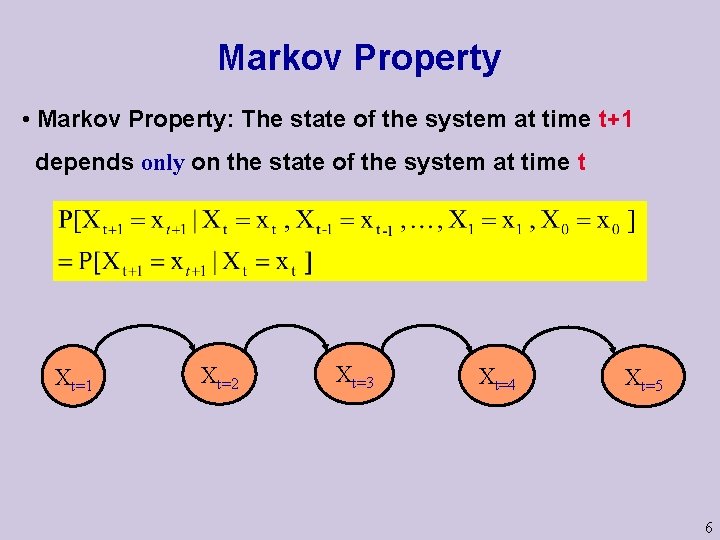
Markov Property • Markov Property: The state of the system at time t+1 depends only on the state of the system at time t Xt=1 Xt=2 Xt=3 Xt=4 Xt=5 6

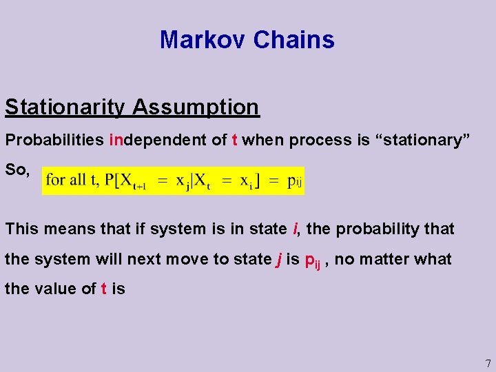
Markov Chains Stationarity Assumption Probabilities independent of t when process is “stationary” So, This means that if system is in state i, the probability that the system will next move to state j is pij , no matter what the value of t is 7

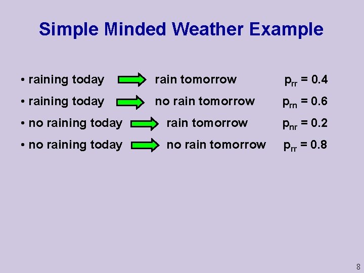
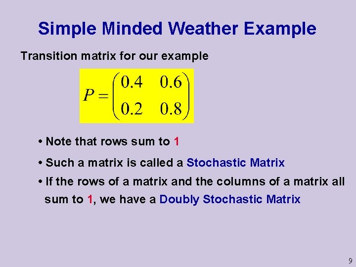
Simple Minded Weather Example • raining today rain tomorrow prr = 0. 4 • raining today no rain tomorrow prn = 0. 6 • no raining today rain tomorrow pnr = 0. 2 • no raining today no rain tomorrow prr = 0. 8 8

Simple Minded Weather Example Transition matrix for our example • Note that rows sum to 1 • Such a matrix is called a Stochastic Matrix • If the rows of a matrix and the columns of a matrix all sum to 1, we have a Doubly Stochastic Matrix 9

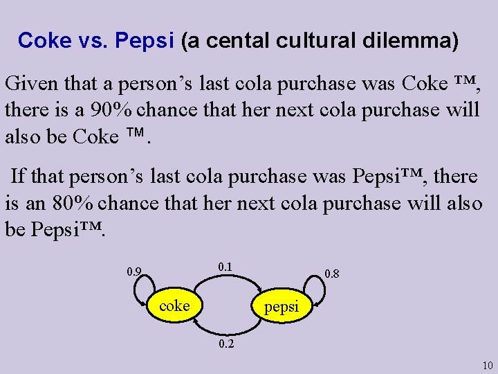
Coke vs. Pepsi (a cental cultural dilemma) Given that a person’s last cola purchase was Coke ™, there is a 90% chance that her next cola purchase will also be Coke ™. If that person’s last cola purchase was Pepsi™, there is an 80% chance that her next cola purchase will also be Pepsi™. 0. 1 0. 9 coke 0. 8 pepsi 0. 2 10

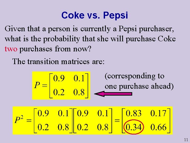
Coke vs. Pepsi Given that a person is currently a Pepsi purchaser, what is the probability that she will purchase Coke two purchases from now? The transition matrices are: (corresponding to one purchase ahead) 11

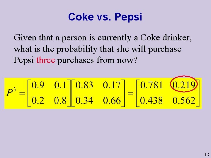
Coke vs. Pepsi Given that a person is currently a Coke drinker, what is the probability that she will purchase Pepsi three purchases from now? 12

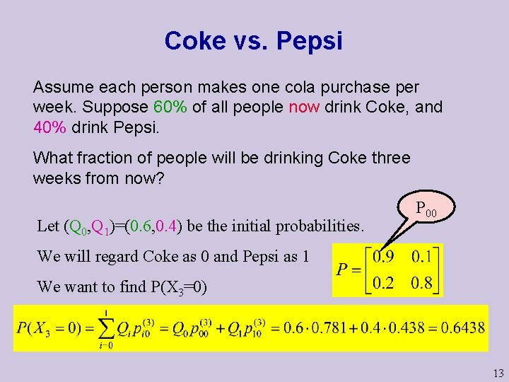
Coke vs. Pepsi Assume each person makes one cola purchase per week. Suppose 60% of all people now drink Coke, and 40% drink Pepsi. What fraction of people will be drinking Coke three weeks from now? Let (Q 0, Q 1)=(0. 6, 0. 4) be the initial probabilities. P 00 We will regard Coke as 0 and Pepsi as 1 We want to find P(X 3=0) 13

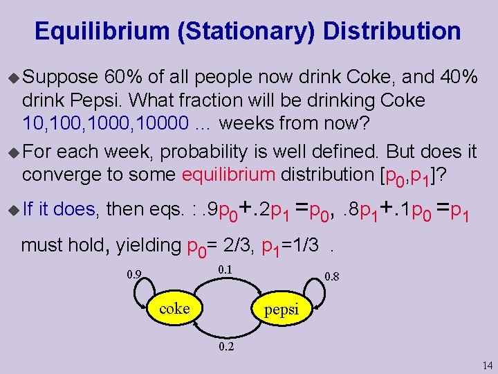
Equilibrium (Stationary) Distribution u Suppose 60% of all people now drink Coke, and 40% drink Pepsi. What fraction will be drinking Coke 10, 1000, 10000 … weeks from now? u For each week, probability is well defined. But does it converge to some equilibrium distribution [p 0, p 1]? u If it does, then eqs. : . 9 p 0+. 2 p 1 =p 0, . 8 p 1+. 1 p 0 =p 1 must hold, yielding p 0= 2/3, p 1=1/3. 0. 1 0. 9 coke 0. 8 pepsi 0. 2 14

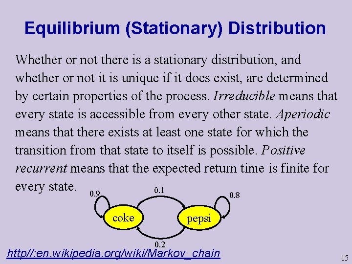
Equilibrium (Stationary) Distribution Whether or not there is a stationary distribution, and whether or not it is unique if it does exist, are determined by certain properties of the process. Irreducible means that every state is accessible from every other state. Aperiodic means that there exists at least one state for which the transition from that state to itself is possible. Positive recurrent means that the expected return time is finite for every state. 0. 9 0. 1 0. 8 coke pepsi 0. 2 http//: en. wikipedia. org/wiki/Markov_chain 15

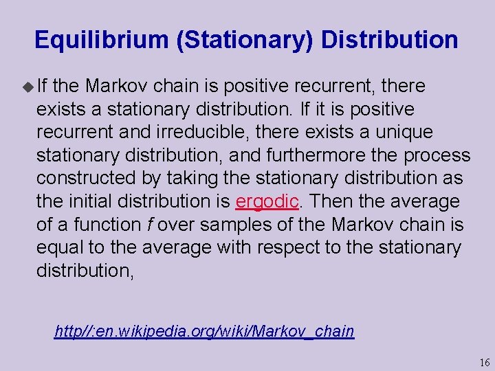
Equilibrium (Stationary) Distribution u If the Markov chain is positive recurrent, there exists a stationary distribution. If it is positive recurrent and irreducible, there exists a unique stationary distribution, and furthermore the process constructed by taking the stationary distribution as the initial distribution is ergodic. Then the average of a function f over samples of the Markov chain is equal to the average with respect to the stationary distribution, http//: en. wikipedia. org/wiki/Markov_chain 16

Equilibrium (Stationary) Distribution u Writing P for the transition matrix, a stationary distribution is a vector π which satisfies the equation l Pπ = π. u In this case, the stationary distribution π is an eigenvector of the transition matrix, associated with the eigenvalue 1. http//: en. wikipedia. org/wiki/Markov_chain 17

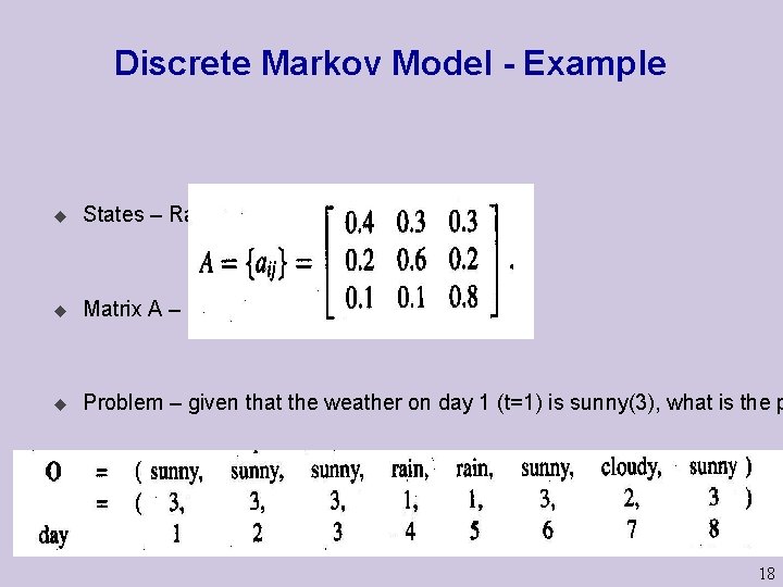
Discrete Markov Model - Example u States – Rainy: 1, Cloudy: 2, Sunny: 3 u Matrix A – u Problem – given that the weather on day 1 (t=1) is sunny(3), what is the p 18

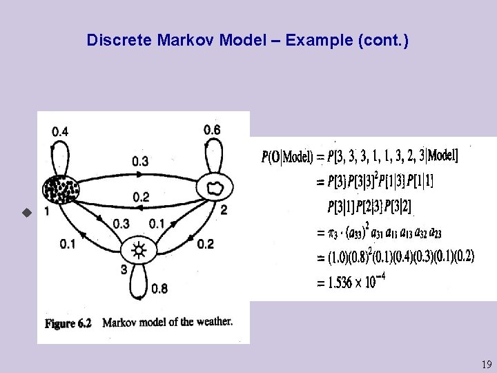
Discrete Markov Model – Example (cont. ) u The answer is - 19

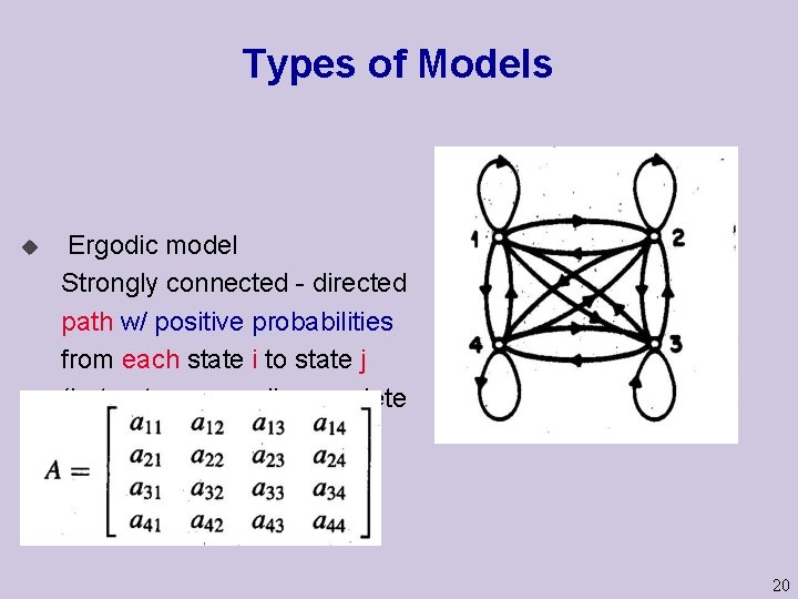
Types of Models u Ergodic model Strongly connected - directed path w/ positive probabilities from each state i to state j (but not necessarily complete directed graph) 20

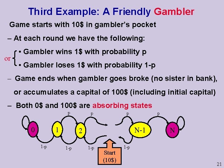
Third Example: A Friendly Gambler Game starts with 10$ in gambler’s pocket – At each round we have the following: or • Gambler wins 1$ with probability p • Gambler loses 1$ with probability 1 -p – Game ends when gambler goes broke (no sister in bank), or accumulates a capital of 100$ (including initial capital) – Both 0$ and 100$ are absorbing states p 0 1 1 -p p p N-1 2 1 -p p 1 -p Start (10$) N 1 -p 21

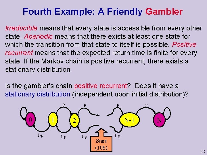
Fourth Example: A Friendly Gambler Irreducible means that every state is accessible from every other state. Aperiodic means that there exists at least one state for which the transition from that state to itself is possible. Positive recurrent means that the expected return time is finite for every state. If the Markov chain is positive recurrent, there exists a stationary distribution. Is the gambler’s chain positive recurrent? Does it have a stationary distribution (independent upon initial distribution)? p 0 1 1 -p p p N-1 2 1 -p p 1 -p Start (10$) N 1 -p 22

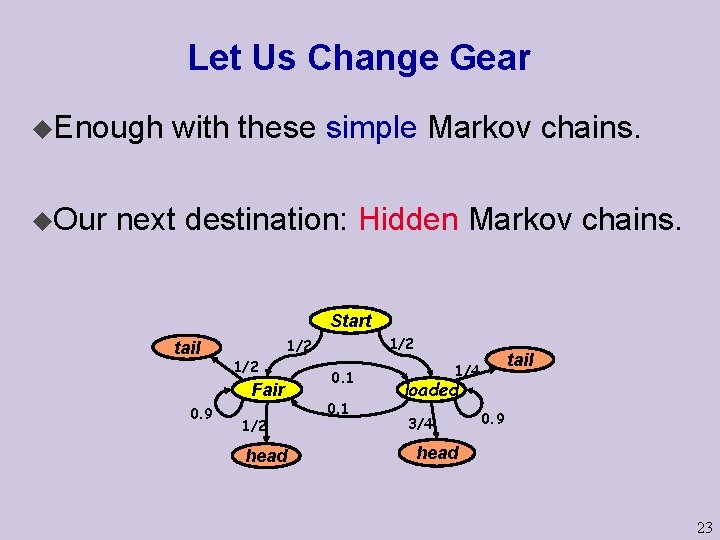
Let Us Change Gear u. Enough u. Our with these simple Markov chains. next destination: Hidden Markov chains. Start tail 1/2 Fair 0. 9 1/2 1/2 head 0. 1 tail 1/4 loaded 3/4 0. 9 head 23

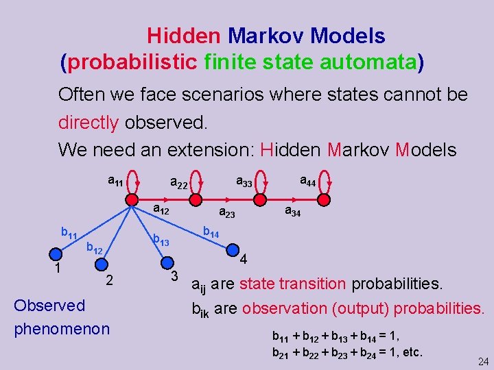
Hidden Markov Models (probabilistic finite state automata) Often we face scenarios where states cannot be directly observed. We need an extension: Hidden Markov Models a 11 a 33 a 22 a 12 b 11 1 a 34 a 23 b 14 b 13 b 12 a 44 4 2 Observed phenomenon 3 aij are state transition probabilities. bik are observation (output) probabilities. b 11 + b 12 + b 13 + b 14 = 1, b 21 + b 22 + b 23 + b 24 = 1, etc. 24

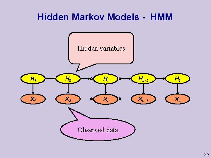
Hidden Markov Models - HMM Hidden variables H 1 H 2 Hi HL-1 HL X 1 X 2 Xi XL-1 XL Observed data 25

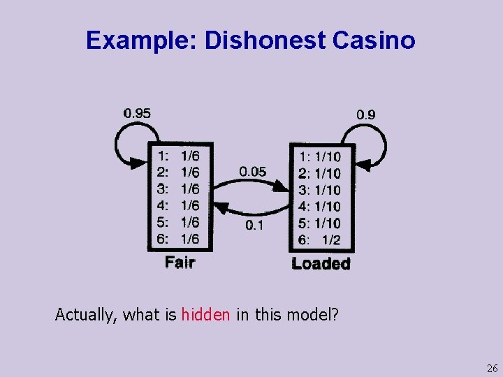
Example: Dishonest Casino Actually, what is hidden in this model? 26

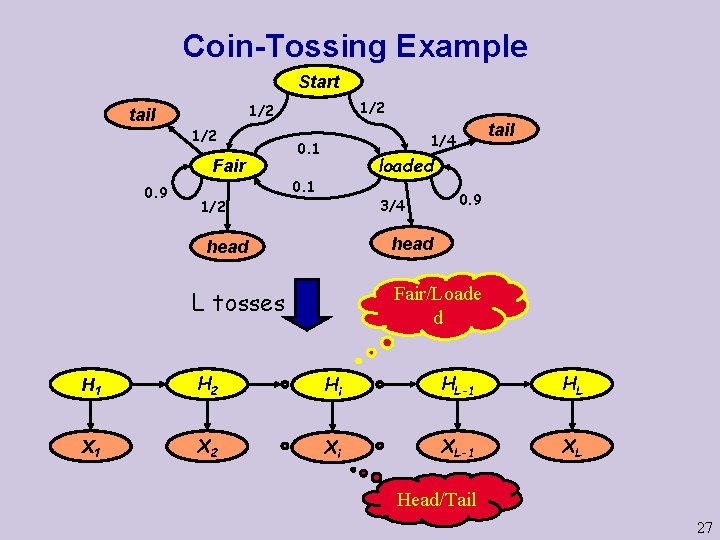
Coin-Tossing Example Start 1/2 Fair 0. 9 1/2 tail 1/4 0. 1 loaded 0. 1 3/4 1/2 0. 9 head Fair/Loade d L tosses H 1 H 2 Hi HL-1 HL X 1 X 2 Xi XL-1 XL Head/Tail 27

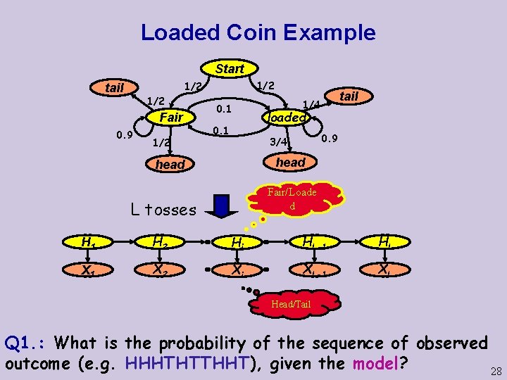
Loaded Coin Example Start 1/2 tail 1/2 Fair 0. 9 1/2 0. 1 tail 1/4 loaded 0. 9 3/4 head Fair/Loade d L tosses H 1 H 2 Hi HL-1 HL X 1 X 2 Xi XL-1 XL Head/Tail Q 1. : What is the probability of the sequence of observed outcome (e. g. HHHTHTTHHT), given the model? 28

HMMs – Question I u Given an observation sequence O = (O 1 O 2 O 3 … OL), and a model M = {A, B, p }, how do we efficiently compute P(O|M), the probability that the given model M produces the observation O in a run of length L ? u This probability can be viewed as a measure of the quality of the model M. Viewed this way, it enables discrimination/selection among alternative models. 29

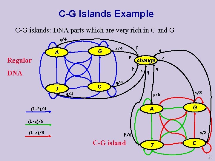
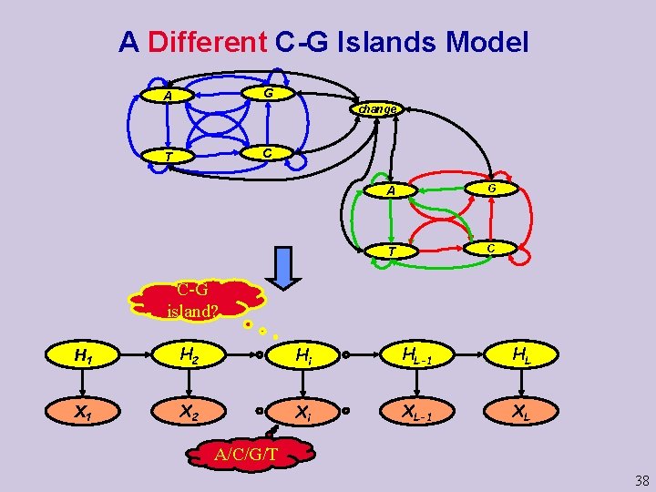
C-G Islands Example C-G islands: DNA parts which are very rich in C and G q/4 G A P q/4 P Regular T C q change P DNA q q P q q/4 p/6 (1 -P)/4 A p/3 G (1 -q)/6 (1 -q)/3 p/3 P/6 C-G island T C 31

Example: Cp. G islands u In human genome, CG dinucleotides are relatively rare l CG pairs undergo a process called methylation that modifies the C nucleotide l A methylated C mutate (with relatively high chance) to a T u Promotor regions are CG rich l l These regions are not methylated, and thus mutate less often These are called Cp. G islands 32

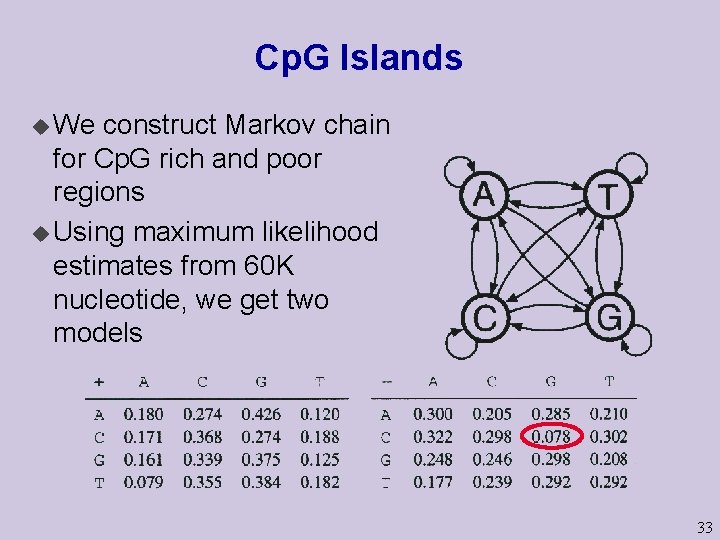
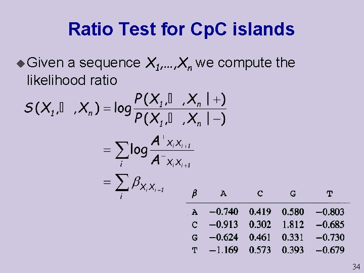
Cp. G Islands u We construct Markov chain for Cp. G rich and poor regions u Using maximum likelihood estimates from 60 K nucleotide, we get two models 33

Ratio Test for Cp. C islands a sequence X 1, …, Xn we compute the likelihood ratio u Given 34

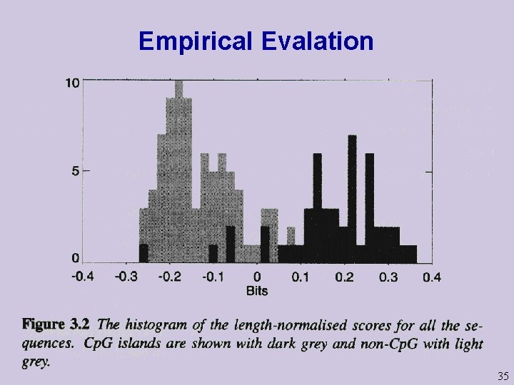
Empirical Evalation 35

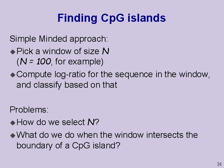
Finding Cp. G islands Simple Minded approach: u Pick a window of size N (N = 100, for example) u Compute log-ratio for the sequence in the window, and classify based on that Problems: u How do we select N? u What do we do when the window intersects the boundary of a Cp. G island? 36

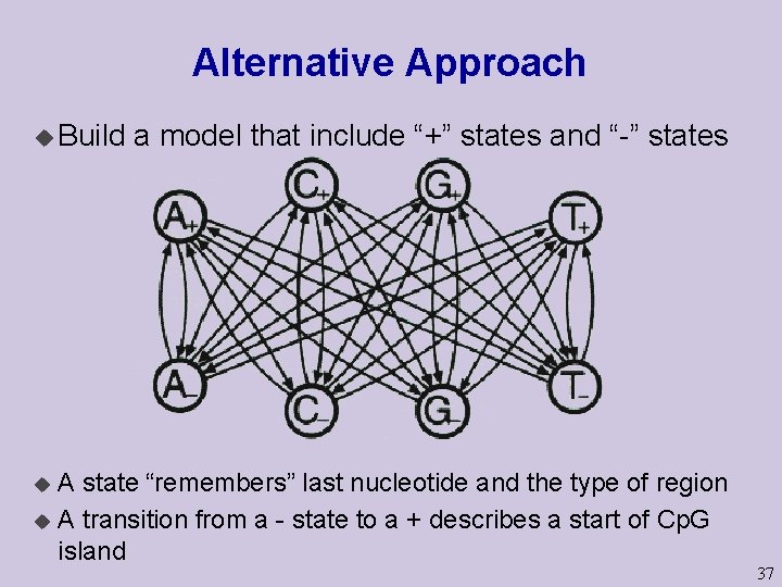
Alternative Approach u Build a model that include “+” states and “-” states A state “remembers” last nucleotide and the type of region u A transition from a - state to a + describes a start of Cp. G island u 37

A Different C-G Islands Model G A change C T A G T C C-G island? H 1 H 2 Hi HL-1 HL X 1 X 2 Xi XL-1 XL A/C/G/T 38

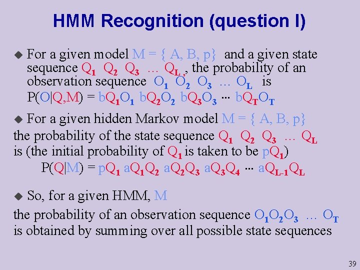
HMM Recognition (question I) u For a given model M = { A, B, p} and a given state sequence Q 1 Q 2 Q 3 … QL , , the probability of an observation sequence O 1 O 2 O 3 … OL is P(O|Q, M) = b. Q 1 O 1 b. Q 2 O 2 b. Q 3 O 3 … b. QTOT For a given hidden Markov model M = { A, B, p} the probability of the state sequence Q 1 Q 2 Q 3 … QL is (the initial probability of Q 1 is taken to be p. Q 1) P(Q|M) = p. Q 1 a. Q 1 Q 2 a. Q 2 Q 3 a. Q 3 Q 4 … a. QL-1 QL u So, for a given HMM, M the probability of an observation sequence O 1 O 2 O 3 … OT is obtained by summing over all possible state sequences u 39

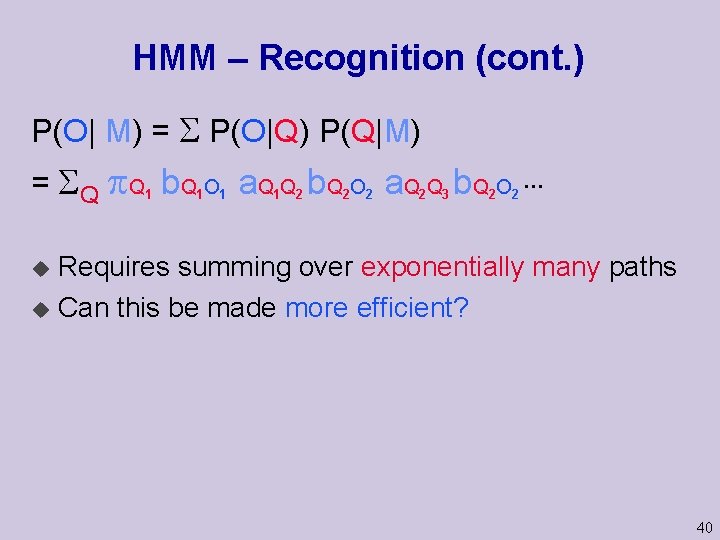
HMM – Recognition (cont. ) P(O| M) = S P(O|Q) P(Q|M) = S Q p Q 1 b. Q 1 O 1 a. Q 1 Q 2 b. Q 2 O 2 a. Q 2 Q 3 b. Q 2 O 2 … Requires summing over exponentially many paths u Can this be made more efficient? u 40

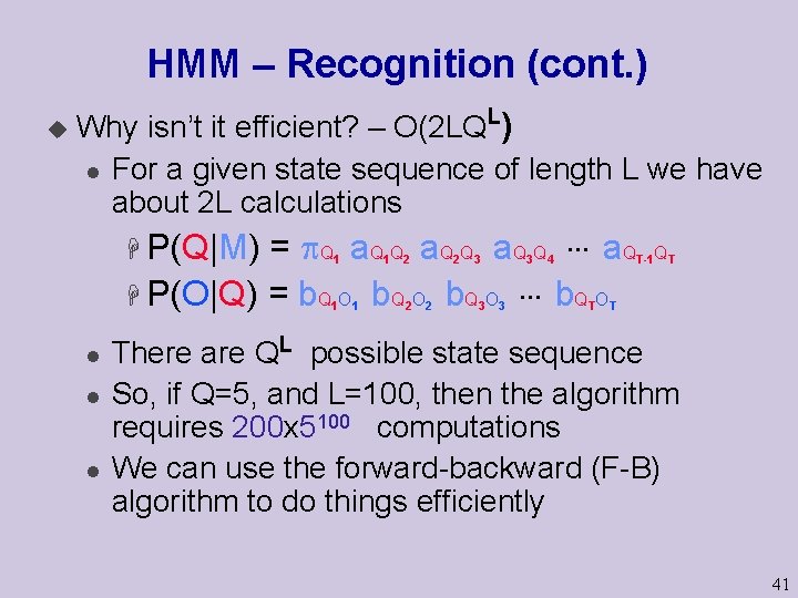
HMM – Recognition (cont. ) u L Why isn’t it efficient? – O(2 LQ ) l For a given state sequence of length L we have about 2 L calculations = p Q a. Q Q … a. Q H P(O|Q) = b. Q O … b. Q O H P(Q|M) 1 1 l l l 1 1 2 2 3 3 4 T T-1 QT T There are QL possible state sequence So, if Q=5, and L=100, then the algorithm requires 200 x 5100 computations We can use the forward-backward (F-B) algorithm to do things efficiently 41

The Forward Backward Algorithm u A white board presentation. 42

The F-B Algorithm (cont. ) Option 1) The likelihood is measured using any sequence of states of length T l This is known as the “Any Path” Method Option 2) We can choose an HMM by the probability generated using the best possible sequence of states l We’ll refer to this method as the “Best Path” Method 43

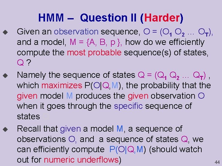
HMM – Question II (Harder) u u u Given an observation sequence, O = (O 1 O 2 … OT), and a model, M = {A, B, p }, how do we efficiently compute the most probable sequence(s) of states, Q? Namely the sequence of states Q = (Q 1 Q 2 … QT) , which maximizes P(O|Q, M), the probability that the given model M produces the given observation O when it goes through the specific sequence of states Q. Recall that given a model M, a sequence of observations O, and a sequence of states Q, we can efficiently compute P(O|Q, M) (should watch out for numeric underflows) 44

Most Probable States Sequence (Q. II) Idea: u If we know the identity of Qi , then the most probable sequence on i+1, …, n does not depend on observations before time i u A white board presentation of Viterbi’s algorithm 45

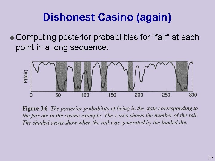
Dishonest Casino (again) u Computing posterior probabilities for “fair” at each point in a long sequence: 46

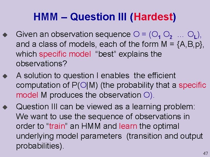
HMM – Question III (Hardest) u u u Given an observation sequence O = (O 1 O 2 … OL), and a class of models, each of the form M = {A, B, p}, which specific model “best” explains the observations? A solution to question I enables the efficient computation of P(O|M) (the probability that a specific model M produces the observation O). Question III can be viewed as a learning problem: We want to use the sequence of observations in order to “train” an HMM and learn the optimal underlying model parameters (transition and output probabilities). 47

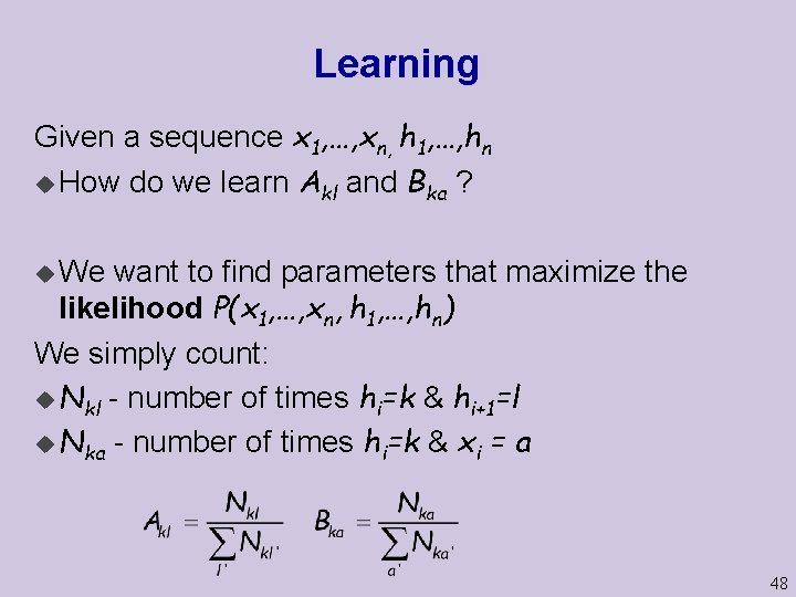
Learning Given a sequence x 1, …, xn, h 1, …, hn u How do we learn Akl and Bka ? u We want to find parameters that maximize the likelihood P(x 1, …, xn, h 1, …, hn) We simply count: u Nkl - number of times hi=k & hi+1=l u Nka - number of times hi=k & xi = a 48

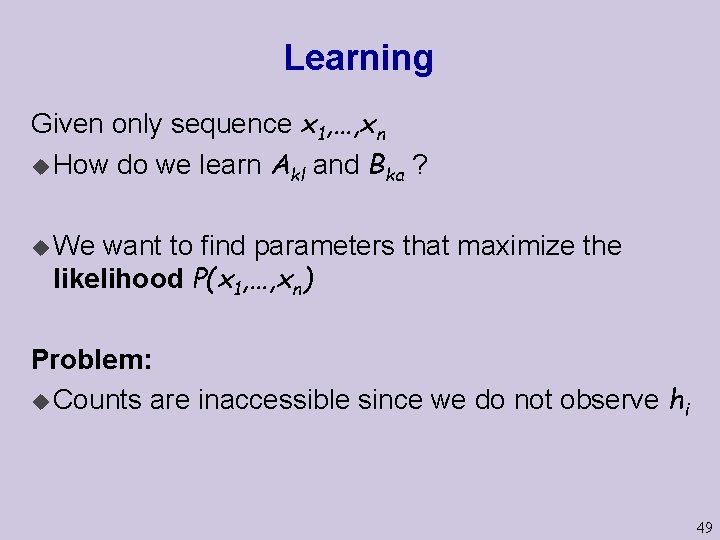
Learning Given only sequence x 1, …, xn u How do we learn Akl and Bka ? u We want to find parameters that maximize the likelihood P(x 1, …, xn) Problem: u Counts are inaccessible since we do not observe hi 49

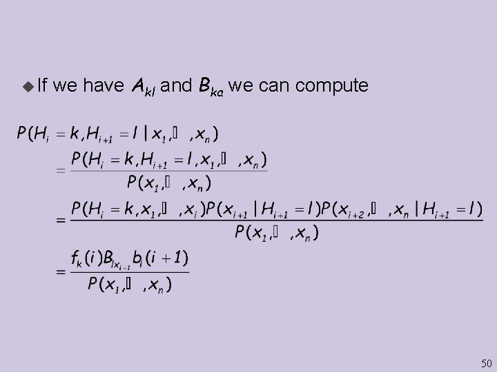
u If we have Akl and Bka we can compute 50

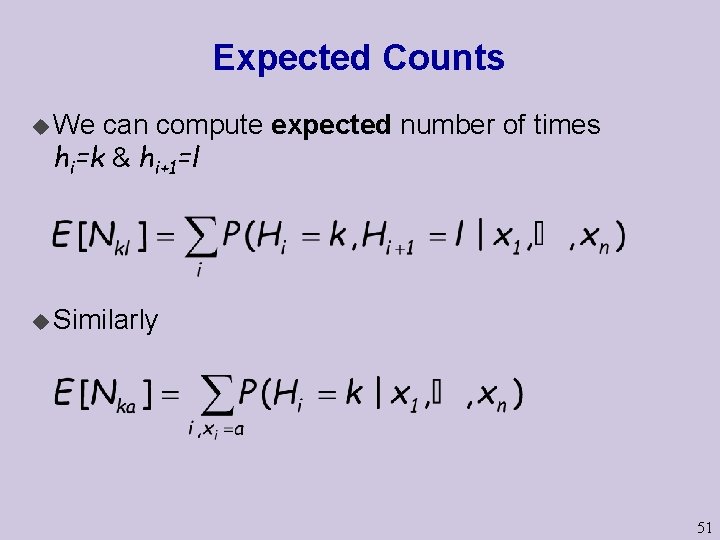
Expected Counts u We can compute expected number of times hi=k & hi+1=l u Similarly 51

Expectation Maximization (EM) u Choose Akl and Bka E-step: u Compute expected counts E[Nkl], E[Nka] M-Step: u Restimate: u Reiterate 52

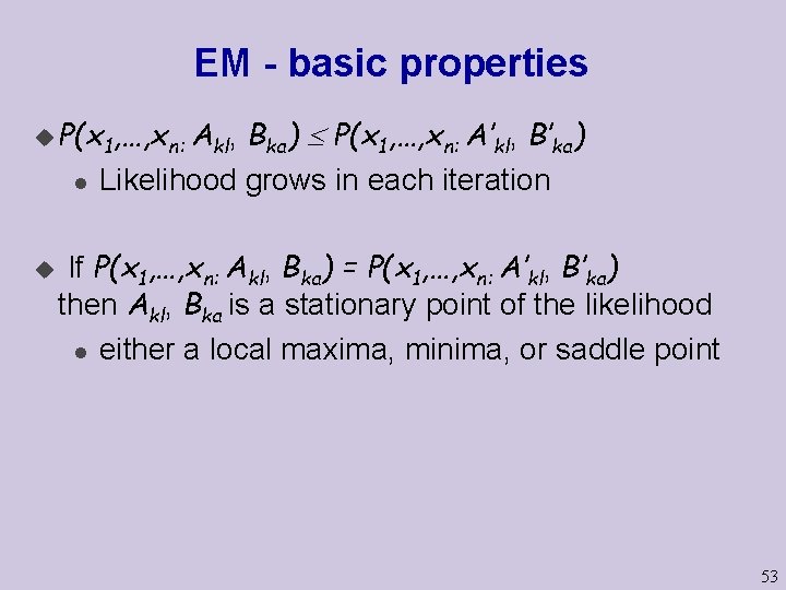
EM - basic properties u P(x 1, …, xn: Akl, l u Bka) P(x 1, …, xn: A’kl, B’ka) Likelihood grows in each iteration If P(x 1, …, xn: Akl, Bka) = P(x 1, …, xn: A’kl, B’ka) then Akl, Bka is a stationary point of the likelihood l either a local maxima, minima, or saddle point 53

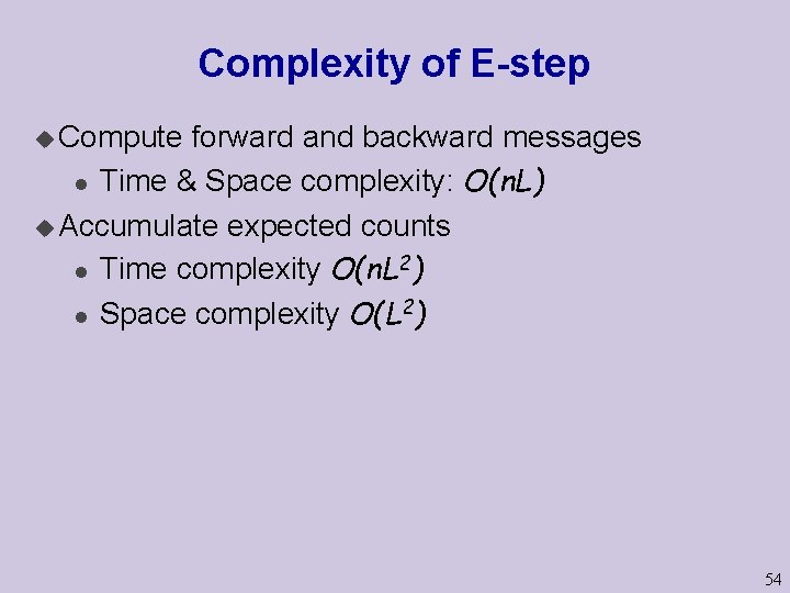
Complexity of E-step u Compute forward and backward messages l Time & Space complexity: O(n. L) u Accumulate expected counts l Time complexity O(n. L 2) l Space complexity O(L 2) 54

EM - problems Local Maxima: u Learning can get stuck in local maxima u Sensitive to initialization u Require some method for escaping such maxima Choosing L u We often do not know how many hidden values we should have or can learn 55

Communication Example 56