Hidden Markov Models Hidden Markov Models HMMs X



- Slides: 16

Hidden Markov Models .

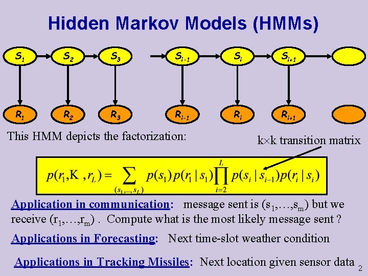
Hidden Markov Models (HMMs) X S 1 X 2 S 2 X 3 S 3 Xi-1 Si-1 Xi Si Xi+1 Si+1 X R 1 X 2 R 2 X 3 R 3 Xi-1 Ri-1 Xi Ri Xi+1 Ri+1 This HMM depicts the factorization: k k transition matrix Application in communication: message sent is (s 1, …, sm) but we receive (r 1, …, rm). Compute what is the most likely message sent ? Applications in Forecasting: Next time-slot weather condition Applications in Tracking Missiles: Next location given sensor data 2

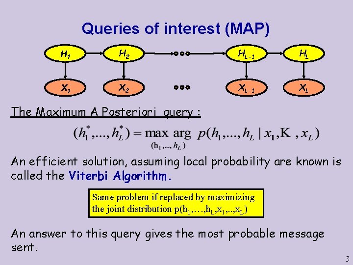
Queries of interest (MAP) H 1 H 2 HL-1 HL X 1 X 2 XL-1 XL The Maximum A Posteriori query : An efficient solution, assuming local probability are known is called the Viterbi Algorithm. Same problem if replaced by maximizing the joint distribution p(h 1, …, h. L, x 1, . . , x. L) An answer to this query gives the most probable message sent. 3

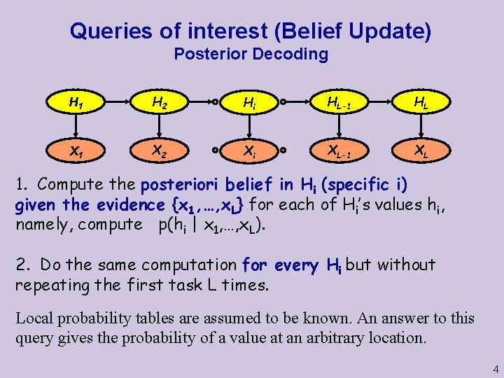
Queries of interest (Belief Update) Posterior Decoding H 1 H 2 Hi HL-1 HL X 1 X 2 Xi XL-1 XL 1. Compute the posteriori belief in Hi (specific i) given the evidence {x 1, …, x. L} for each of Hi’s values hi, namely, compute p(hi | x 1, …, x. L). 2. Do the same computation for every Hi but without repeating the first task L times. Local probability tables are assumed to be known. An answer to this query gives the probability of a value at an arbitrary location. 4

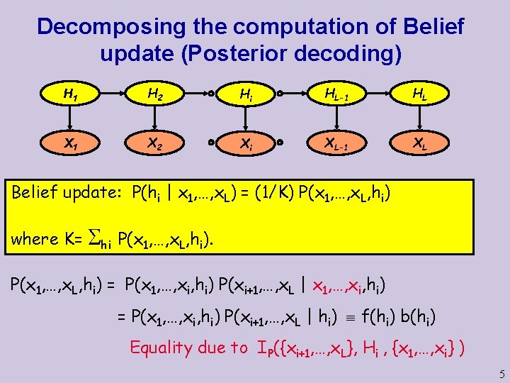
Decomposing the computation of Belief update (Posterior decoding) H 1 H 2 Hi HL-1 HL X 1 X 2 Xi XL-1 XL Belief update: P(hi | x 1, …, x. L) = (1/K) P(x 1, …, x. L, hi) where K= hi P(x 1, …, x. L, hi) = P(x 1, …, xi, hi) P(xi+1, …, x. L | x 1, …, xi, hi) = P(x 1, …, xi, hi) P(xi+1, …, x. L | hi) f(hi) b(hi) Equality due to IP({xi+1, …, x. L}, Hi , {x 1, …, xi} ) 5

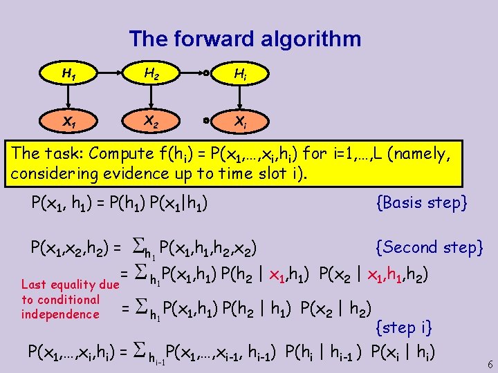
The forward algorithm H 1 H 2 Hi X 1 X 2 Xi The task: Compute f(hi) = P(x 1, …, xi, hi) for i=1, …, L (namely, considering evidence up to time slot i). P(x 1, h 1) = P(h 1) P(x 1|h 1) h P(x 1, h 2, x 2) = h P(x 1, h 1) P(h 2 | x 1, h 1) Last equality due P(x 1, x 2, h 2) = 1 1 to conditional independence {Basis step} {Second step} P(x 2 | x 1, h 2) = h P(x 1, h 1) P(h 2 | h 1) P(x 2 | h 2) 1 {step i} P(x 1, …, xi, hi) = hi-1 P(x 1, …, xi-1, hi-1) P(hi | hi-1 ) P(xi | hi) 6

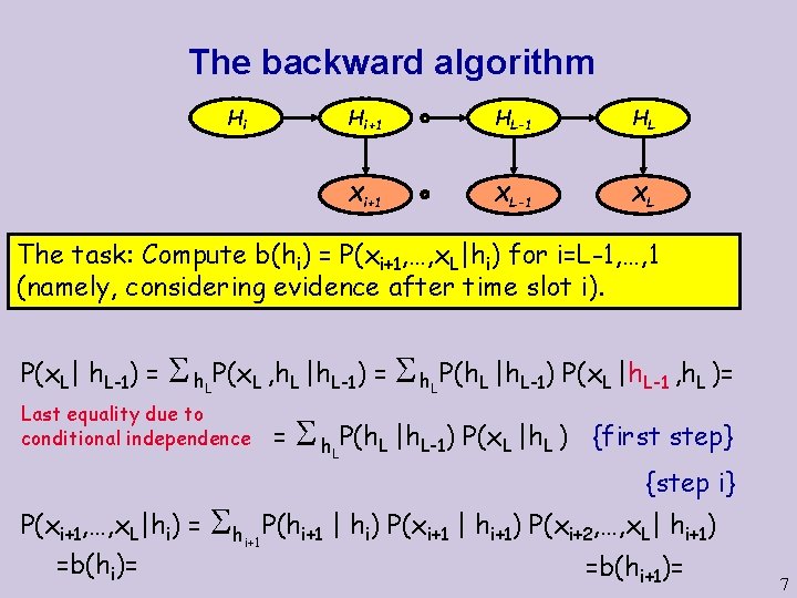
The backward algorithm Hi Hi+1 HL-1 HL Xi+1 XL-1 XL The task: Compute b(hi) = P(xi+1, …, x. L|hi) for i=L-1, …, 1 (namely, considering evidence after time slot i). P(x. L| h. L-1) = h P(x. L , h. L |h. L-1) = h P(h. L |h. L-1) P(x. L |h. L-1 , h. L )= L L Last equality due to conditional independence P(xi+1, …, x. L|hi) = =b(hi)= h. LP(h. L |h. L-1) P(x. L |h. L ) {first step} {step i} i+1 P(hi+1 | hi) P(xi+1 | hi+1) P(xi+2, …, x. L| hi+1) =b(hi+1)= 7

The combined answer H 1 H 2 Hi HL-1 HL X 1 X 2 Xi XL-1 XL 1. To Compute the posteriori belief in Hi (specific i) given the evidence {x 1, …, x. L} run the forward algorithm and compute f(hi) = P(x 1, …, xi, hi), run the backward algorithm to compute b(hi) = P(xi+1, …, x. L|hi), the product f(hi)b(hi) is the answer (for every possible value hi). 2. To Compute the posteriori belief for every Hi simply run the forward and backward algorithms once, storing f(hi) and b(hi) for every i (and value hi). Compute f(hi)b(hi) for every i. 8

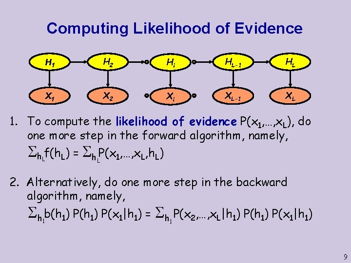
Computing Likelihood of Evidence H 1 H 2 Hi HL-1 HL X 1 X 2 Xi XL-1 XL 1. To compute the likelihood of evidence P(x 1, …, x. L), do one more step in the forward algorithm, namely, h. Lf(h. L) = h. LP(x 1, …, x. L, h. L) 2. Alternatively, do one more step in the backward algorithm, namely, h b(h 1) P(x 1|h 1) = h P(x 2, …, x. L|h 1) P(x 1|h 1) 1 1 9

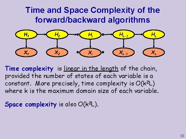
Time and Space Complexity of the forward/backward algorithms H 1 H 2 Hi HL-1 HL X 1 X 2 Xi XL-1 XL Time complexity is linear in the length of the chain, provided the number of states of each variable is a constant. More precisely, time complexity is O(k 2 L) where k is the maximum domain size of each variable. Space complexity is also O(k 2 L). 10

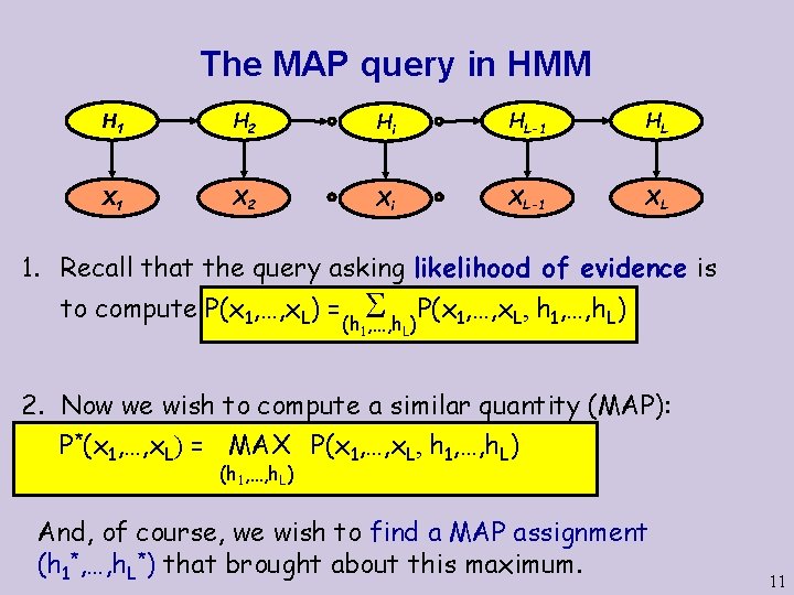
The MAP query in HMM H 1 H 2 Hi HL-1 HL X 1 X 2 Xi XL-1 XL 1. Recall that the query asking likelihood of evidence is to compute P(x 1, …, x. L) = (h 1, …, h. L) P(x 1, …, x. L, h 1, …, h. L) 2. Now we wish to compute a similar quantity (MAP): P*(x 1, …, x. L) = MAX P(x 1, …, x. L, h 1, …, h. L) (h 1, …, h. L) And, of course, we wish to find a MAP assignment (h 1*, …, h. L*) that brought about this maximum. 11

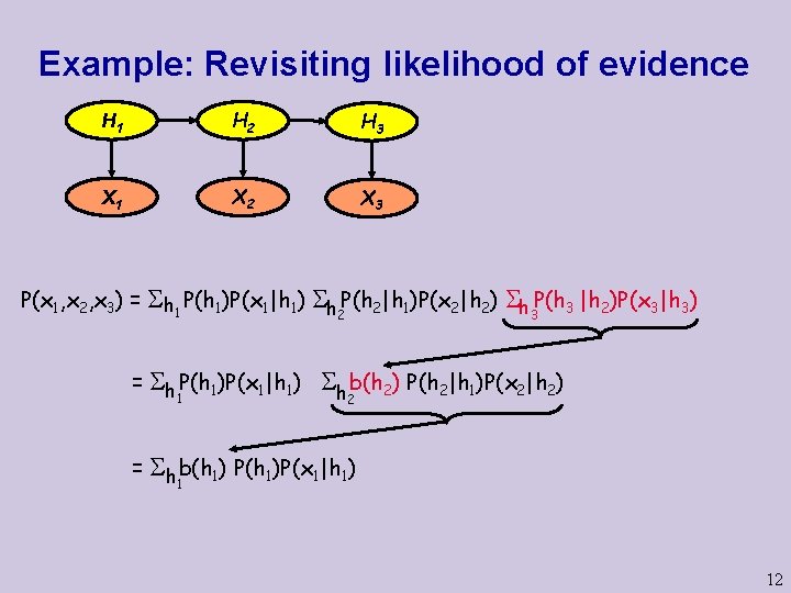
Example: Revisiting likelihood of evidence H 1 H 2 H 3 X 1 X 2 X 3 P(x 1, x 2, x 3) = h 1 P(h 1)P(x 1|h 1) h 2 P(h 2|h 1)P(x 2|h 2) h 3 P(h 3 |h 2)P(x 3|h 3) = h P(h 1)P(x 1|h 1) 1 = h b(h 2) P(h 2|h 1)P(x 2|h 2) 2 h b(h 1) P(h 1)P(x 1|h 1) 1 12

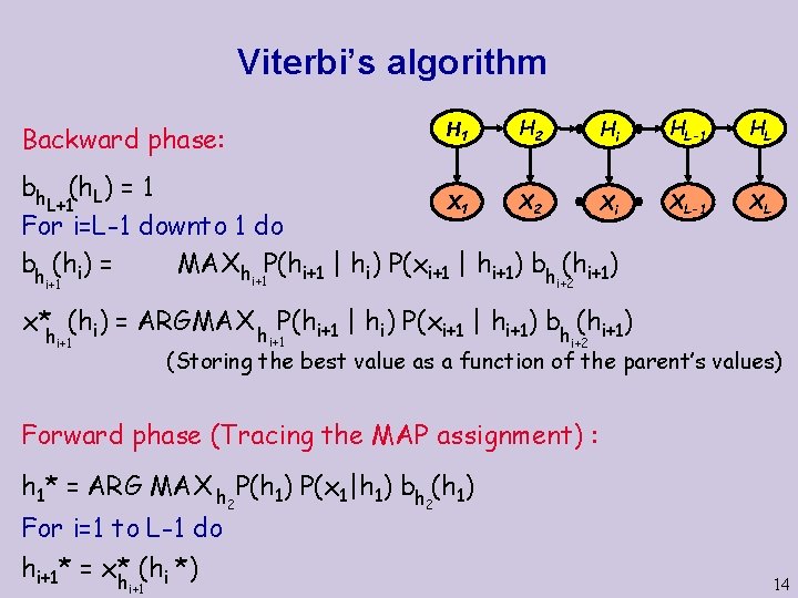
Example: Computing the MAP assignment H 1 H 2 H 3 X 1 X 2 X 3 Replace sums with taking maximum: maximum = max h P(h 1)P(x 1|h 1) max P(h 2|h 1)P(x 2|h 2) max P(h 3 |h 2)P(x 3|h 3) h 3 h 2 1 = max P(h 1)P(x 1|h 1) max b (h 2) P(h 1|h 2)P(x 2|h 2) h 2 h 3 h 1 = max b (h 1) P(h 1)P(x 1|h 1) h 1 h 2 h 1 * = arg max b h(h 1) P(h 1)P(x 1|h 1) h 1 2 h 2* = x* (h 1*); h 3* = x* (h 2*) h 2 h 3 x* h 3 (h 2) x* h 2 (h 1) {Finding the maximum} {Finding the map assignment} 13

Viterbi’s algorithm H 1 Backward phase: H 2 Hi bh (h. L) = 1 X 2 X 1 Xi L+1 For i=L-1 downto 1 do bh (hi) = MAX h P(hi+1 | hi) P(xi+1 | hi+1) bh (hi+1) i+1 HL-1 HL XL-1 XL i+2 x*h (hi) = ARGMAX h P(hi+1 | hi) P(xi+1 | hi+1) bh (hi+1) i+1 i+2 (Storing the best value as a function of the parent’s values) Forward phase (Tracing the MAP assignment) : h 1* = ARG MAX h P(h 1) P(x 1|h 1) bh (h 1) For i=1 to L-1 do hi+1* = x* (hi *) h i+1 2 2 14

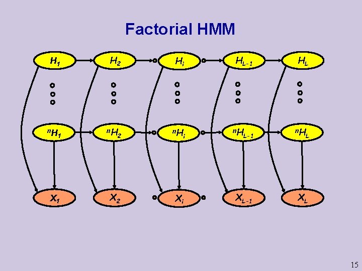
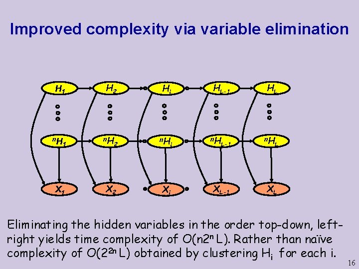
Factorial HMM H 1 n. H 1 X 1 H 2 n. H Hi 2 n. H X 2 Xi i HL-1 n. H L-1 XL-1 HL n. H L XL 15

Improved complexity via variable elimination H 1 n. H 1 X 1 H 2 n. H Hi 2 n. H X 2 Xi i HL-1 n. H L-1 XL-1 HL n. H L XL Eliminating the hidden variables in the order top-down, leftright yields time complexity of O(n 2 n L). Rather than naïve complexity of O(22 n L) obtained by clustering Hi for each i. 16