Hidden Markov Models HMMs 1 Definition Hidden Markov

Hidden Markov Models (HMMs) 1

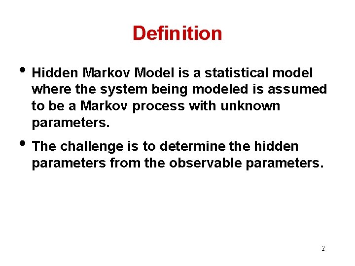
Definition • Hidden Markov Model is a statistical model where the system being modeled is assumed to be a Markov process with unknown parameters. • The challenge is to determine the hidden parameters from the observable parameters. 2

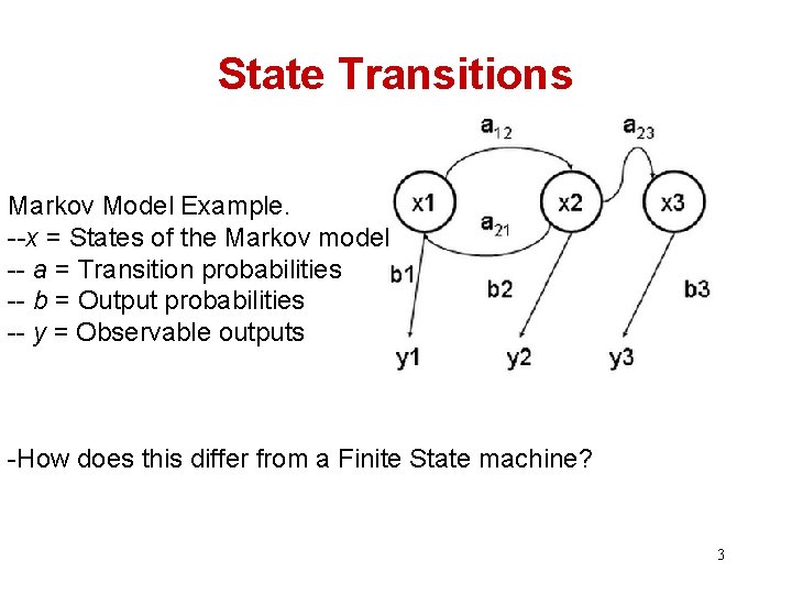
State Transitions Markov Model Example. --x = States of the Markov model -- a = Transition probabilities -- b = Output probabilities -- y = Observable outputs -How does this differ from a Finite State machine? 3

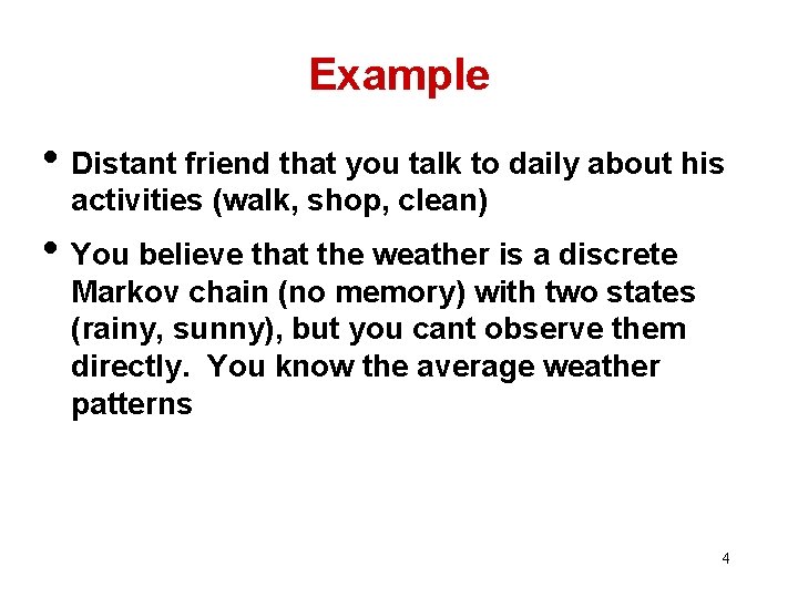
Example • Distant friend that you talk to daily about his activities (walk, shop, clean) • You believe that the weather is a discrete Markov chain (no memory) with two states (rainy, sunny), but you cant observe them directly. You know the average weather patterns 4

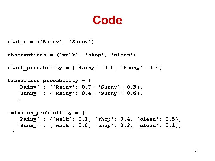
Code states = ('Rainy', 'Sunny') observations = ('walk', 'shop', 'clean') start_probability = {'Rainy': 0. 6, 'Sunny': 0. 4} transition_probability = { 'Rainy' : {'Rainy': 0. 7, 'Sunny': 0. 3}, 'Sunny' : {'Rainy': 0. 4, 'Sunny': 0. 6}, } emission_probability = { 'Rainy' : {'walk': 0. 1, 'shop': 0. 4, 'clean': 0. 5}, 'Sunny' : {'walk': 0. 6, 'shop': 0. 3, 'clean': 0. 1}, } 5

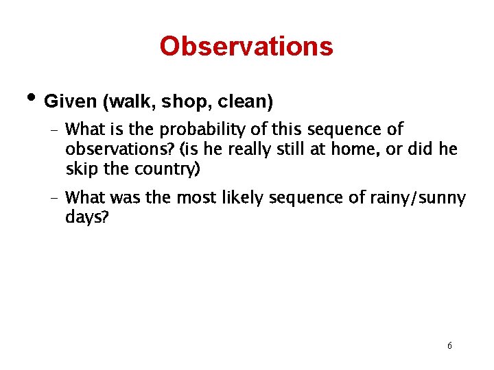
Observations • Given (walk, shop, clean) – What is the probability of this sequence of observations? (is he really still at home, or did he skip the country) – What was the most likely sequence of rainy/sunny days? 6

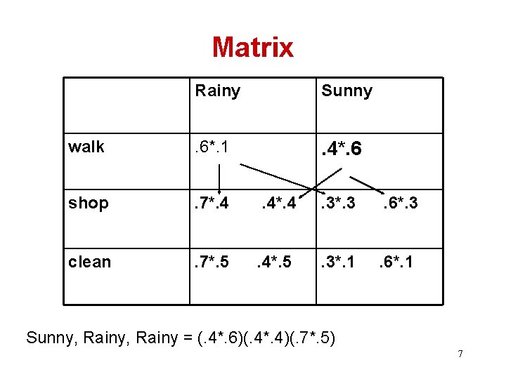
Matrix Rainy Sunny walk . 6*. 1 . 4*. 6 shop . 7*. 4 . 4*. 4 . 3*. 3 . 6*. 3 clean . 7*. 5 . 4*. 5 . 3*. 1 . 6*. 1 Sunny, Rainy = (. 4*. 6)(. 4*. 4)(. 7*. 5) 7

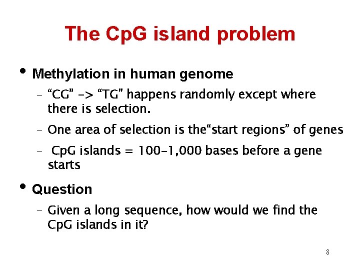
The Cp. G island problem • Methylation in human genome – “CG” -> “TG” happens randomly except where there is selection. – One area of selection is the“start regions” of genes – Cp. G islands = 100 -1, 000 bases before a gene starts • Question – Given a long sequence, how would we find the Cp. G islands in it? 8

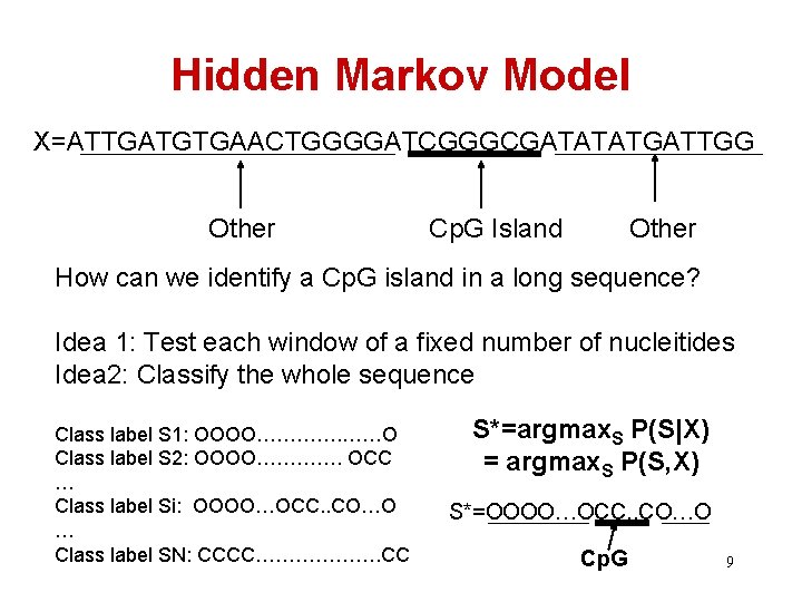
Hidden Markov Model X=ATTGATGTGAACTGGGGATCGGGCGATATATGATTGG Other Cp. G Island Other How can we identify a Cp. G island in a long sequence? Idea 1: Test each window of a fixed number of nucleitides Idea 2: Classify the whole sequence Class label S 1: OOOO…………. ……O Class label S 2: OOOO…………. OCC … Class label Si: OOOO…OCC. . CO…O … Class label SN: CCCC………………. CC S*=argmax. S P(S|X) = argmax. S P(S, X) S*=OOOO…OCC. . CO…O Cp. G 9

HMM is just one way of modeling p(X, S)… 10

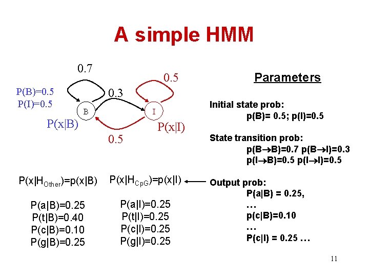
A simple HMM 0. 7 P(B)=0. 5 P(I)=0. 5 Parameters 0. 3 B I P(x|B) 0. 5 P(x|I) P(x|HOther)=p(x|B) P(x|HCp. G)=p(x|I) P(a|B)=0. 25 P(t|B)=0. 40 P(c|B)=0. 10 P(g|B)=0. 25 P(a|I)=0. 25 P(t|I)=0. 25 P(c|I)=0. 25 P(g|I)=0. 25 Initial state prob: p(B)= 0. 5; p(I)=0. 5 State transition prob: p(B B)=0. 7 p(B I)=0. 3 p(I B)=0. 5 p(I I)=0. 5 Output prob: P(a|B) = 0. 25, … p(c|B)=0. 10 … P(c|I) = 0. 25 … 11

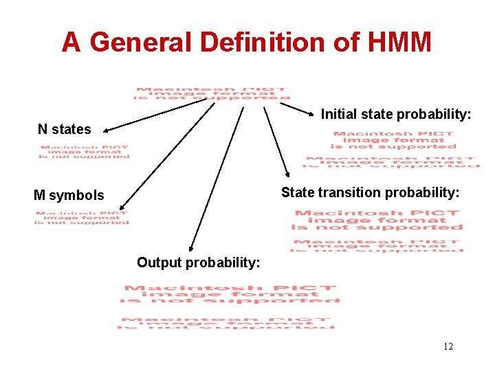
A General Definition of HMM Initial state probability: N states State transition probability: M symbols Output probability: 12

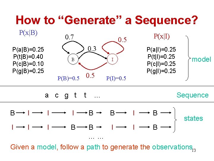
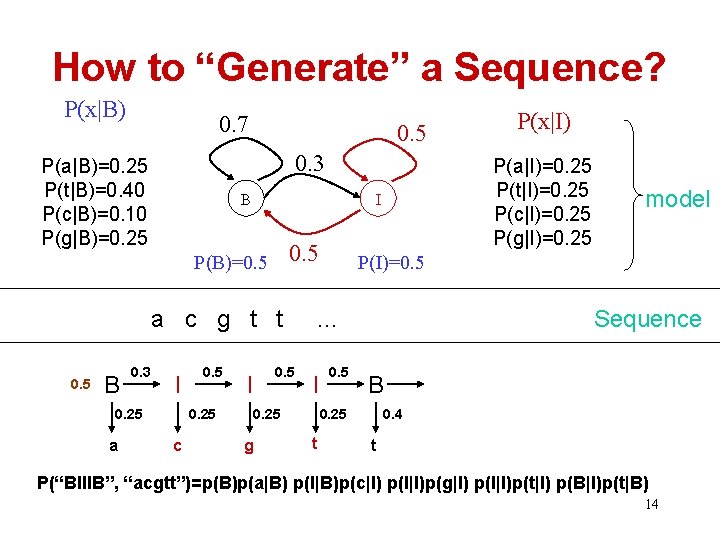
How to “Generate” a Sequence? P(x|B) 0. 7 P(x|I) 0. 5 0. 3 P(a|B)=0. 25 P(t|B)=0. 40 P(c|B)=0. 10 P(g|B)=0. 25 B P(B)=0. 5 a c g t B I I I B P(a|I)=0. 25 P(t|I)=0. 25 P(c|I)=0. 25 P(g|I)=0. 25 I 0. 5 t P(I)=0. 5 … B model Sequence B I B states B I I B …… Given a model, follow a path to generate the observations. 13

How to “Generate” a Sequence? P(x|B) 0. 7 0. 5 0. 3 P(a|B)=0. 25 P(t|B)=0. 40 P(c|B)=0. 10 P(g|B)=0. 25 B 0. 5 a c g t t 0. 5 B 0. 3 I 0. 25 a 0. 5 0. 25 c P(a|I)=0. 25 P(t|I)=0. 25 P(c|I)=0. 25 P(g|I)=0. 25 I P(B)=0. 5 I 0. 25 g 0. 5 Sequence B 0. 25 t model P(I)=0. 5 … I P(x|I) 0. 4 t P(“BIIIB”, “acgtt”)=p(B)p(a|B) p(I|B)p(c|I) p(I|I)p(g|I) p(I|I)p(t|I) p(B|I)p(t|B) 14

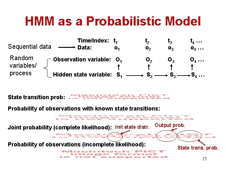
HMM as a Probabilistic Model Time/Index: t 1 Data: o 1 t 2 o 2 t 3 o 3 t 4 … o 4 … Observation variable: O 1 O 2 O 3 O 4 … Hidden state variable: S 1 S 2 S 3 S 4 … Sequential data Random variables/ process State transition prob: Probability of observations with known state transitions: Joint probability (complete likelihood): Init state distr. Output prob. Probability of observations (incomplete likelihood): State trans. prob. 15

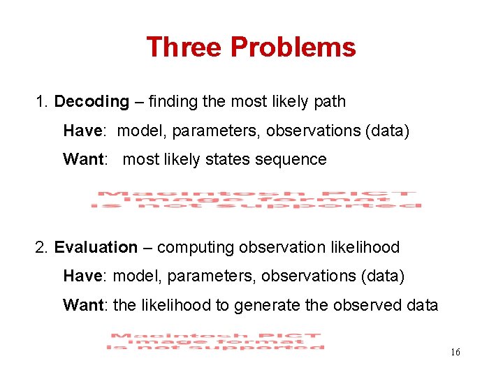
Three Problems 1. Decoding – finding the most likely path Have: model, parameters, observations (data) Want: most likely states sequence 2. Evaluation – computing observation likelihood Have: model, parameters, observations (data) Want: the likelihood to generate the observed data 16

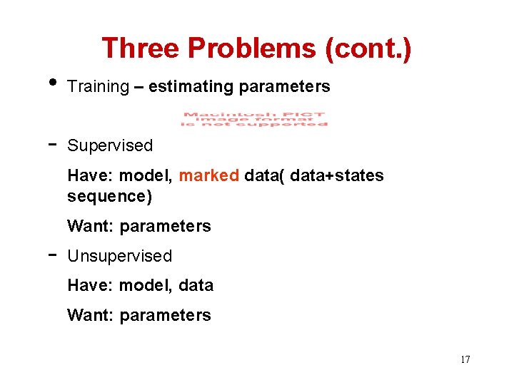
Three Problems (cont. ) • Training – estimating parameters - Supervised Have: model, marked data( data+states sequence) Want: parameters - Unsupervised Have: model, data Want: parameters 17

Problem I: Decoding/Parsing Finding the most likely path You can think of this as classification with all the paths as class labels… 18

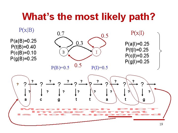
What’s the most likely path? P(x|B) 0. 7 P(a|B)=0. 25 P(t|B)=0. 40 P(c|B)=0. 10 P(g|B)=0. 25 0. 3 B ? ? a ? ? c ? ? 0. 5 ? ? ? g P(a|I)=0. 25 P(t|I)=0. 25 P(c|I)=0. 25 P(g|I)=0. 25 I P(B)=0. 5 ? P(x|I) 0. 5 P(I)=0. 5 ? ? t ? ? ? a ? ? ? t ? g 19

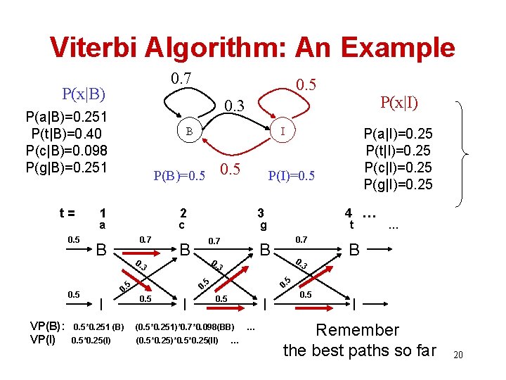
Viterbi Algorithm: An Example 0. 7 P(x|B) 0. 5 B VP(B): VP(I) I 0. 5 P(B)=0. 5 1 a 3 c 0. 7 B 0. 3 I 0. 7 t 0. 7 B 0. B 5 5 0. I … 3 3 0. 5 4 … g B P(a|I)=0. 25 P(t|I)=0. 25 P(c|I)=0. 25 P(g|I)=0. 25 P(I)=0. 5 2 5 0. 5 P(x|I) 0. 3 P(a|B)=0. 251 P(t|B)=0. 40 P(c|B)=0. 098 P(g|B)=0. 251 t= 0. 5 I 0. 5*0. 251 (B) (0. 5*0. 251)*0. 7*0. 098(BB) 0. 5*0. 25(I) (0. 5*0. 25)*0. 5*0. 25(II) … … 0. 5 I Remember the best paths so far 20

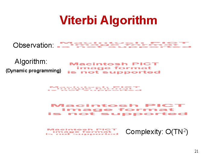
Viterbi Algorithm Observation: Algorithm: (Dynamic programming) Complexity: O(TN 2) 21

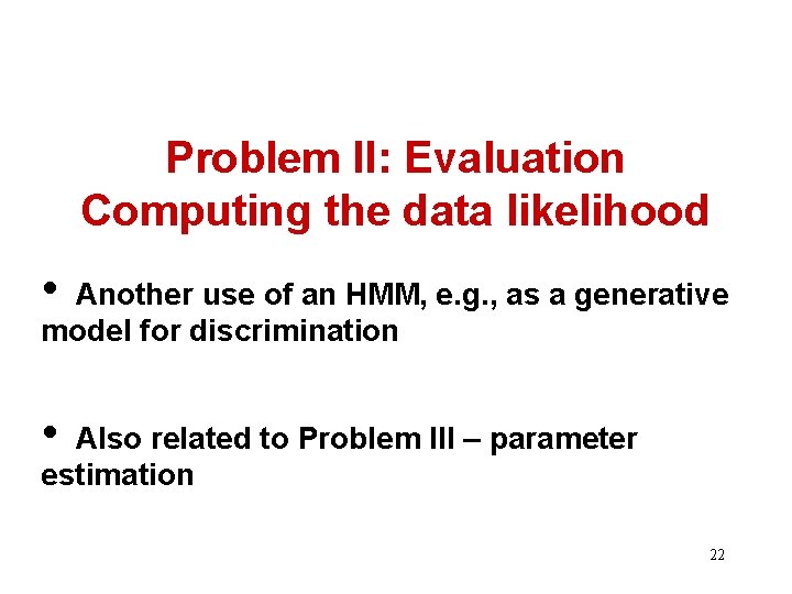
Problem II: Evaluation Computing the data likelihood • Another use of an HMM, e. g. , as a generative model for discrimination • Also related to Problem III – parameter estimation 22

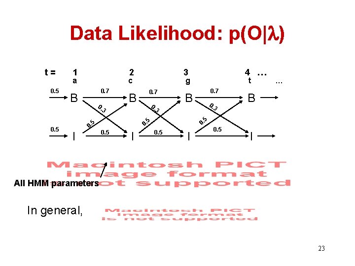
Data Likelihood: p(O| ) t= 0. 5 1 2 a c 0. 7 B 0. 3 I 0. 7 0. t 0. 7 B 0. 3 3 I … B 5 5 0. 0. 5 4 … g B 5 0. 5 3 0. 5 I All HMM parameters In general, 23

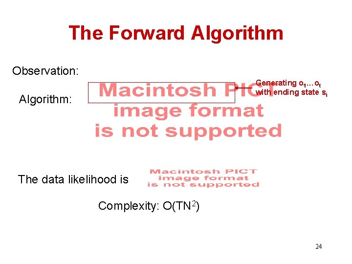
The Forward Algorithm Observation: Generating o 1…ot with ending state si Algorithm: The data likelihood is Complexity: O(TN 2) 24

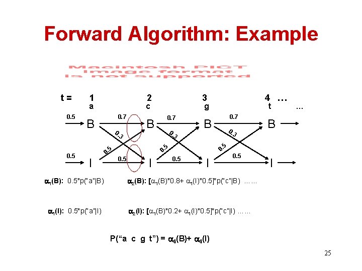
Forward Algorithm: Example t= 0. 5 1 2 a c 0. 7 B 0. 3 I 1(B): 0. 5*p(“a”|B) 1(I): 0. 5*p(“a”|I) 0. 7 0. t 0. 7 B 0. 3 3 I … B 5 5 0. 0. 5 4 … g B 5 0. 5 3 0. 5 I 2(B): [ 1(B)*0. 8+ 1(I)*0. 5]*p(“c”|B) …… 2(I): [ 1(B)*0. 2+ 1(I)*0. 5]*p(“c”|I) …… P(“a c g t”) = 4(B)+ 4(I) 25

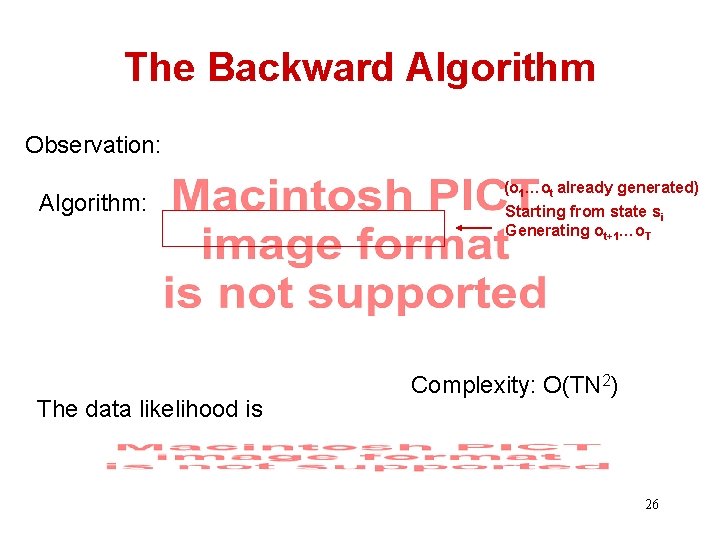
The Backward Algorithm Observation: Algorithm: The data likelihood is (o 1…ot already generated) Starting from state si Generating ot+1…o. T Complexity: O(TN 2) 26

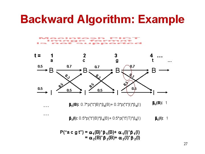
Backward Algorithm: Example t= 0. 5 1 2 a c 0. 7 B 0. 3 … … 0. 7 0. t 0. 7 B 0. 3 3 5 I 4 … g B I B 5 0. 0. 5 … 0. 5 0. 5 3 0. 5 I 3(B): 0. 7*p(“t”|B)* 4(B)+ 0. 3*p(“t”|I)* 4(I) 4(B): 1 3(I): 0. 5*p(“t”|B)* 4(B)+ 0. 5*p(“t”|T)* 4(I): 1 P(“a c g t”) = 1(B)* 1(B)+ 1(I)* 1(I) = 2(B)* 2(B)+ 2(I)* 2(I) 27

Problem III: Training Estimating Parameters Where do we get the probability values for all parameters? Supervised vs. Unsupervised 28

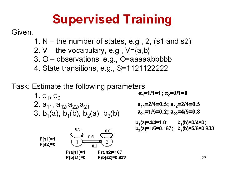
Supervised Training Given: 1. N – the number of states, e. g. , 2, (s 1 and s 2) 2. V – the vocabulary, e. g. , V={a, b} 3. O – observations, e. g. , O=aaaaabbbbb 4. State transitions, e. g. , S=1121122222 Task: Estimate the following parameters 1=1/1=1; 2=0/1=0 1. 1, 2 a 11=2/4=0. 5; a 12=2/4=0. 5 2. a 11, a 12, a 21=1/5=0. 2; a 22=4/5=0. 8 3. b 1(a), b 1(b), b 2(a), b 2(b) 0. 5 P(s 1)=1 P(s 2)=0 0. 8 b 1(a)=4/4=1. 0; b 1(b)=0/4=0; b 2(a)=1/6=0. 167; b 2(b)=5/6=0. 833 0. 5 1 P(a|s 1)=1 P(b|s 1)=0 0. 2 2 P(a|s 2)=167 P(b|s 2)=0. 833 29

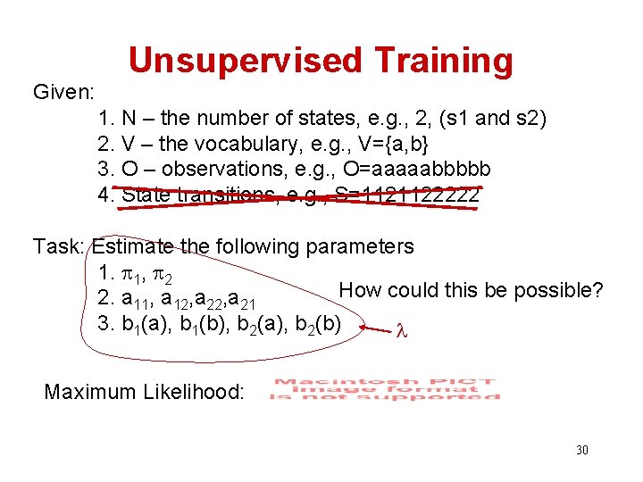
Given: Unsupervised Training 1. N – the number of states, e. g. , 2, (s 1 and s 2) 2. V – the vocabulary, e. g. , V={a, b} 3. O – observations, e. g. , O=aaaaabbbbb 4. State transitions, e. g. , S=1121122222 Task: Estimate the following parameters 1. 1, 2 How could this be possible? 2. a 11, a 12, a 21 3. b 1(a), b 1(b), b 2(a), b 2(b) Maximum Likelihood: 30

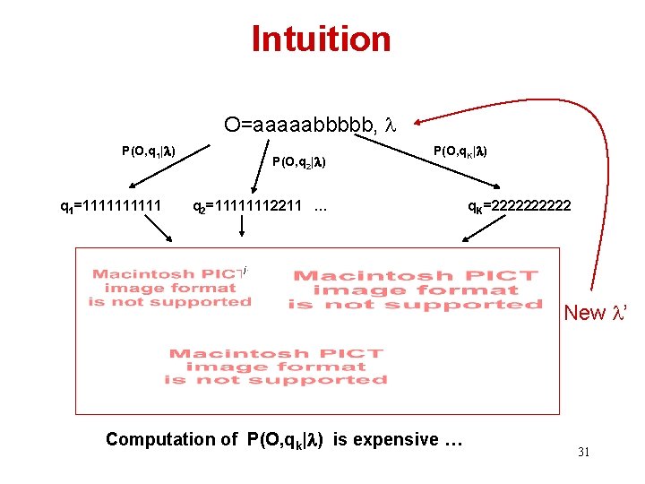
Intuition O=aaaaabbbbb, P(O, q 1| ) q 1=11111 P(O, q 2| ) P(O, q. K| ) q 2=11111112211 … q. K=22222 i New ’ Computation of P(O, qk| ) is expensive … 31

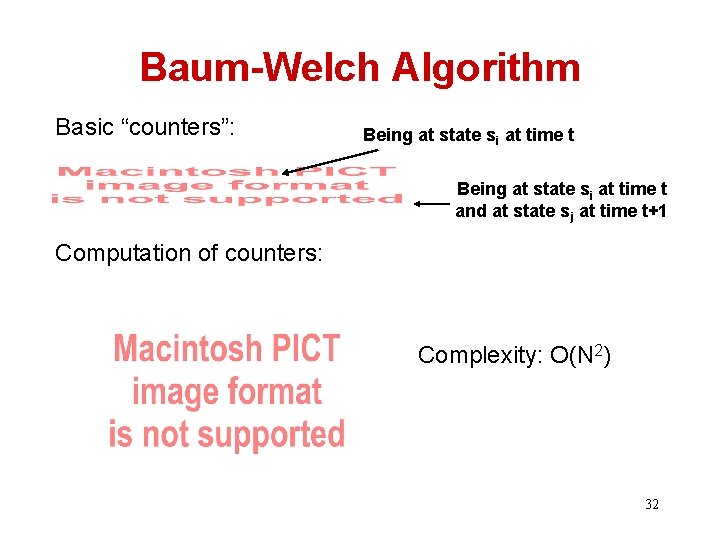
Baum-Welch Algorithm Basic “counters”: Being at state si at time t and at state sj at time t+1 Computation of counters: Complexity: O(N 2) 32

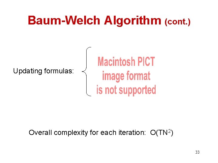
Baum-Welch Algorithm (cont. ) Updating formulas: Overall complexity for each iteration: O(TN 2) 33

Next Time • Tutorial • Posted on blackboard 34