Hidden Markov Models HMMs Lecture for CS 498

Hidden Markov Models (HMMs) (Lecture for CS 498 -CXZ Algorithms in Bioinformatics) Oct. 27, 2005 Cheng. Xiang Zhai Department of Computer Science University of Illinois, Urbana-Champaign 1

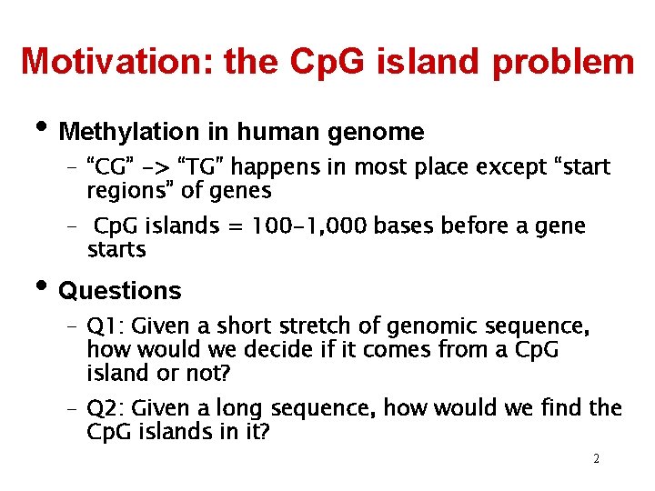
Motivation: the Cp. G island problem • Methylation in human genome – “CG” -> “TG” happens in most place except “start regions” of genes – Cp. G islands = 100 -1, 000 bases before a gene starts • Questions – Q 1: Given a short stretch of genomic sequence, how would we decide if it comes from a Cp. G island or not? – Q 2: Given a long sequence, how would we find the Cp. G islands in it? 2

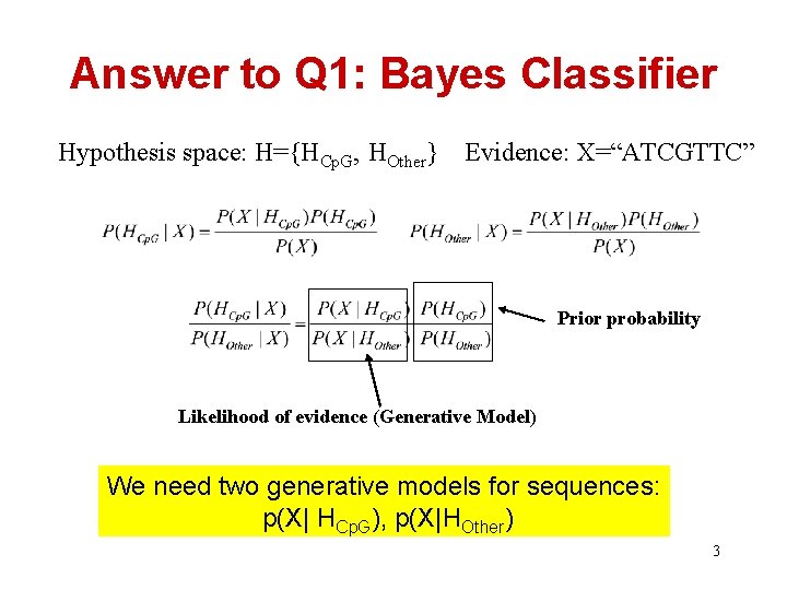
Answer to Q 1: Bayes Classifier Hypothesis space: H={HCp. G, HOther} Evidence: X=“ATCGTTC” Prior probability Likelihood of evidence (Generative Model) We need two generative models for sequences: p(X| HCp. G), p(X|HOther) 3

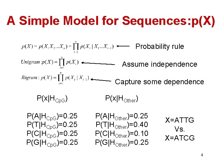
A Simple Model for Sequences: p(X) Probability rule Assume independence Capture some dependence P(x|HCp. G) P(x|HOther) P(A|HCp. G)=0. 25 P(T|HCp. G)=0. 25 P(C|HCp. G)=0. 25 P(G|HCp. G)=0. 25 P(A|HOther)=0. 25 P(T|HOther)=0. 40 P(C|HOther)=0. 10 P(G|HOther)=0. 25 X=ATTG Vs. X=ATCG 4

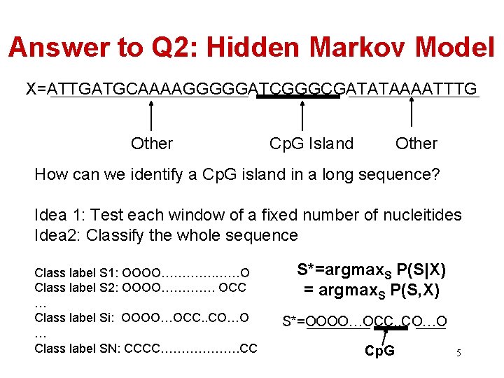
Answer to Q 2: Hidden Markov Model X=ATTGATGCAAAAGGGGGATCGGGCGATATAAAATTTG Other Cp. G Island Other How can we identify a Cp. G island in a long sequence? Idea 1: Test each window of a fixed number of nucleitides Idea 2: Classify the whole sequence Class label S 1: OOOO…………. ……O Class label S 2: OOOO…………. OCC … Class label Si: OOOO…OCC. . CO…O … Class label SN: CCCC………………. CC S*=argmax. S P(S|X) = argmax. S P(S, X) S*=OOOO…OCC. . CO…O Cp. G 5

HMM is just one way of modeling p(X, S)… 6

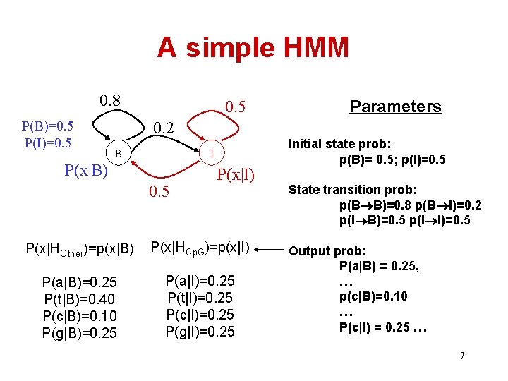
A simple HMM 0. 8 P(B)=0. 5 P(I)=0. 5 Parameters 0. 2 B I P(x|B) 0. 5 P(x|I) P(x|HOther)=p(x|B) P(x|HCp. G)=p(x|I) P(a|B)=0. 25 P(t|B)=0. 40 P(c|B)=0. 10 P(g|B)=0. 25 P(a|I)=0. 25 P(t|I)=0. 25 P(c|I)=0. 25 P(g|I)=0. 25 Initial state prob: p(B)= 0. 5; p(I)=0. 5 State transition prob: p(B B)=0. 8 p(B I)=0. 2 p(I B)=0. 5 p(I I)=0. 5 Output prob: P(a|B) = 0. 25, … p(c|B)=0. 10 … P(c|I) = 0. 25 … 7

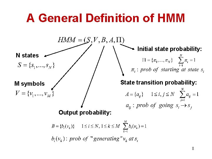
A General Definition of HMM Initial state probability: N states State transition probability: M symbols Output probability: 8

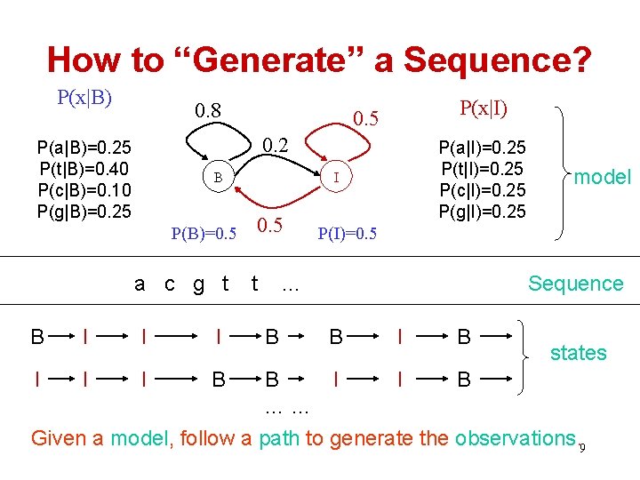
How to “Generate” a Sequence? P(x|B) 0. 8 P(x|I) 0. 5 0. 2 P(a|B)=0. 25 P(t|B)=0. 40 P(c|B)=0. 10 P(g|B)=0. 25 B P(B)=0. 5 a c g t B I I I B P(a|I)=0. 25 P(t|I)=0. 25 P(c|I)=0. 25 P(g|I)=0. 25 I 0. 5 t P(I)=0. 5 … B model Sequence B I B states B I I B …… Given a model, follow a path to generate the observations. 9

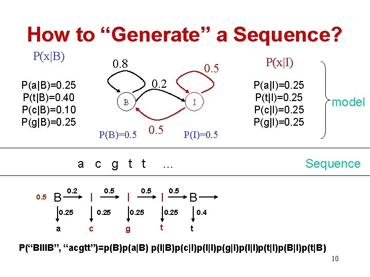
How to “Generate” a Sequence? P(x|B) 0. 8 0. 5 0. 2 P(a|B)=0. 25 P(t|B)=0. 40 P(c|B)=0. 10 P(g|B)=0. 25 B 0. 5 a c g t t 0. 5 B 0. 2 I 0. 25 a 0. 5 0. 25 c P(a|I)=0. 25 P(t|I)=0. 25 P(c|I)=0. 25 P(g|I)=0. 25 I P(B)=0. 5 I 0. 5 0. 25 g 0. 5 Sequence B 0. 25 t model P(I)=0. 5 … I P(x|I) 0. 4 t P(“BIIIB”, “acgtt”)=p(B)p(a|B) p(I|B)p(c|I)p(I|I)p(g|I)p(I|I)p(t|I)p(B|I)p(t|B) 10

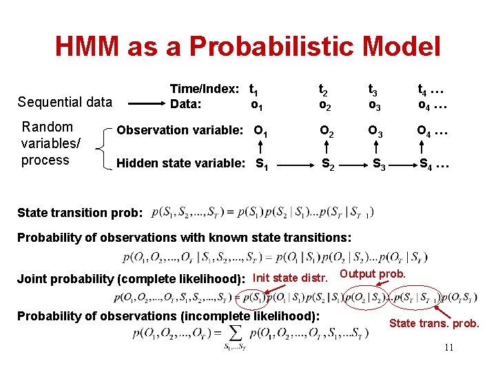
HMM as a Probabilistic Model Time/Index: t 1 Data: o 1 t 2 o 2 t 3 o 3 t 4 … o 4 … Observation variable: O 1 O 2 O 3 O 4 … Hidden state variable: S 1 S 2 S 3 S 4 … Sequential data Random variables/ process State transition prob: Probability of observations with known state transitions: Joint probability (complete likelihood): Init state distr. Output prob. Probability of observations (incomplete likelihood): State trans. prob. 11

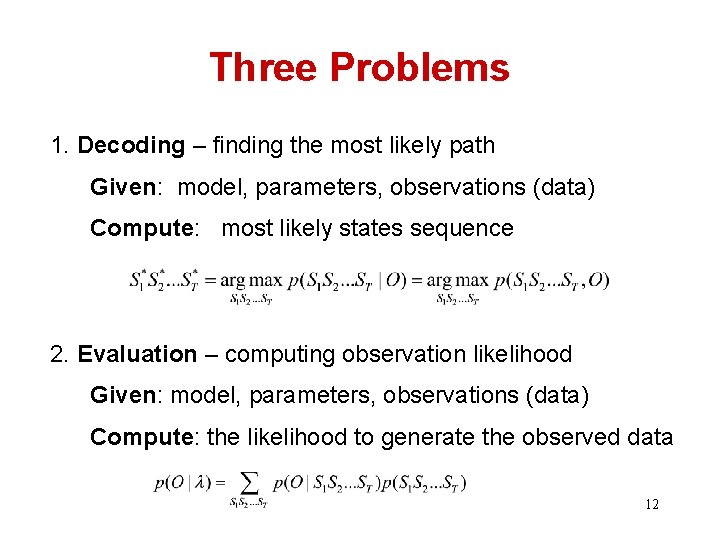
Three Problems 1. Decoding – finding the most likely path Given: model, parameters, observations (data) Compute: most likely states sequence 2. Evaluation – computing observation likelihood Given: model, parameters, observations (data) Compute: the likelihood to generate the observed data 12

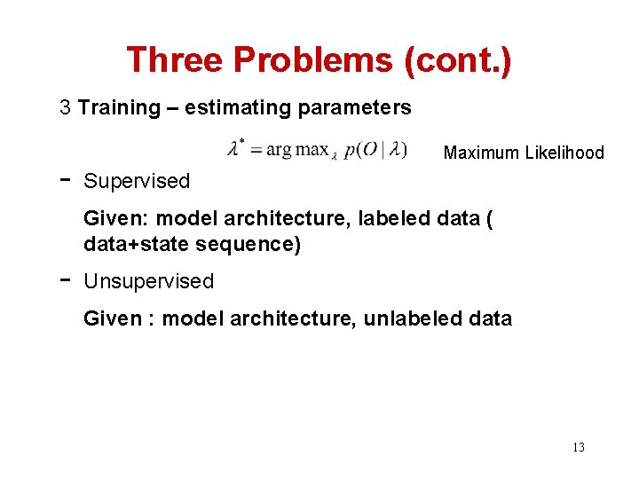
Three Problems (cont. ) 3 Training – estimating parameters - Maximum Likelihood Supervised Given: model architecture, labeled data ( data+state sequence) - Unsupervised Given : model architecture, unlabeled data 13

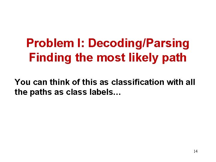
Problem I: Decoding/Parsing Finding the most likely path You can think of this as classification with all the paths as class labels… 14

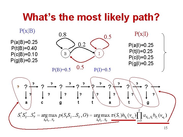
What’s the most likely path? P(x|B) 0. 8 P(a|B)=0. 25 P(t|B)=0. 40 P(c|B)=0. 10 P(g|B)=0. 25 0. 2 B ? ? a ? ? c ? ? 0. 5 ? ? ? g P(a|I)=0. 25 P(t|I)=0. 25 P(c|I)=0. 25 P(g|I)=0. 25 I P(B)=0. 5 ? P(x|I) 0. 5 P(I)=0. 5 ? ? t ? ? ? a ? ? ? t ? g 15

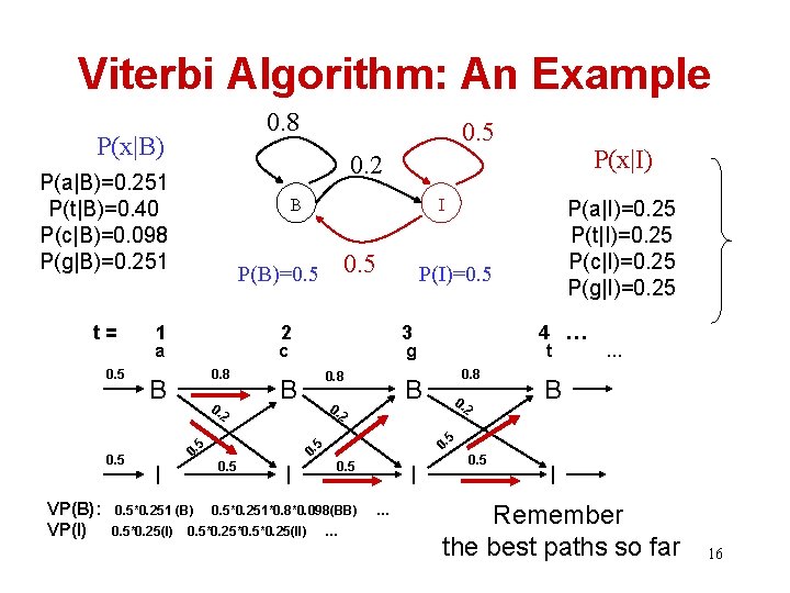
Viterbi Algorithm: An Example 0. 8 P(x|B) 0. 5 B VP(B): VP(I) 1 0. 5 2 a 0. 8 0. 2 B I 0. 5*0. 251 (B) t 0. 8 B 0. 2 2 I B 5 0. 5*0. 251*0. 8*0. 098(BB) 0. 5*0. 25*0. 25(II) … 0. 5 0. 0. 5 4 … g 0. 8 P(a|I)=0. 25 P(t|I)=0. 25 P(c|I)=0. 25 P(g|I)=0. 25 P(I)=0. 5 3 c B 0. 5*0. 25(I) I P(B)=0. 5 5 0. 5 P(x|I) 0. 2 P(a|B)=0. 251 P(t|B)=0. 40 P(c|B)=0. 098 P(g|B)=0. 251 t= 0. 5 … I … 0. 5 I Remember the best paths so far 16

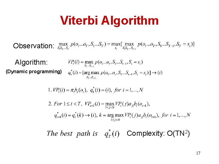
Viterbi Algorithm Observation: Algorithm: (Dynamic programming) Complexity: O(TN 2) 17

Problem II: Evaluation Computing the data likelihood • Another use of an HMM, e. g. , as a generative model for discrimination • Also related to Problem III – parameter estimation 18

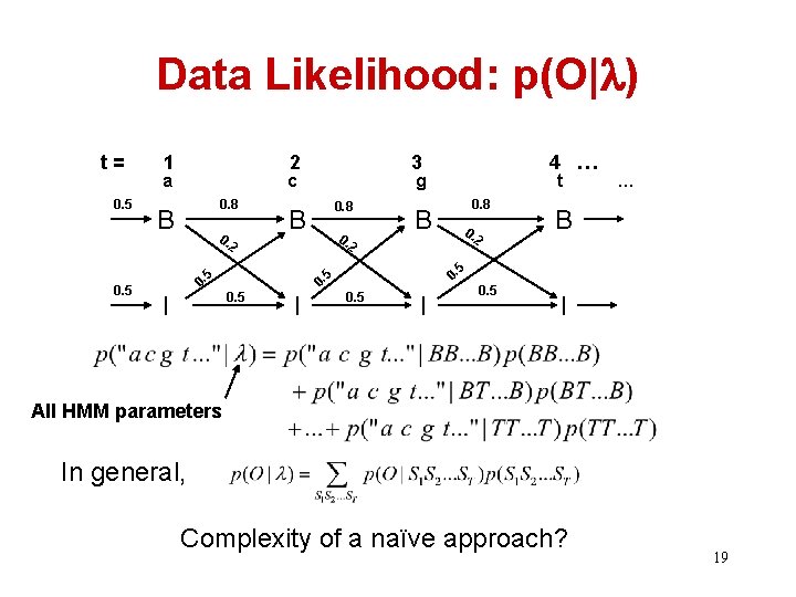
Data Likelihood: p(O| ) t= 0. 5 1 2 a c 0. 8 B 0. 2 I 0. 8 0. t 0. 8 B 0. 2 2 I … B 5 0. 0. 5 4 … g B 5 0. 5 3 0. 5 I All HMM parameters In general, Complexity of a naïve approach? 19

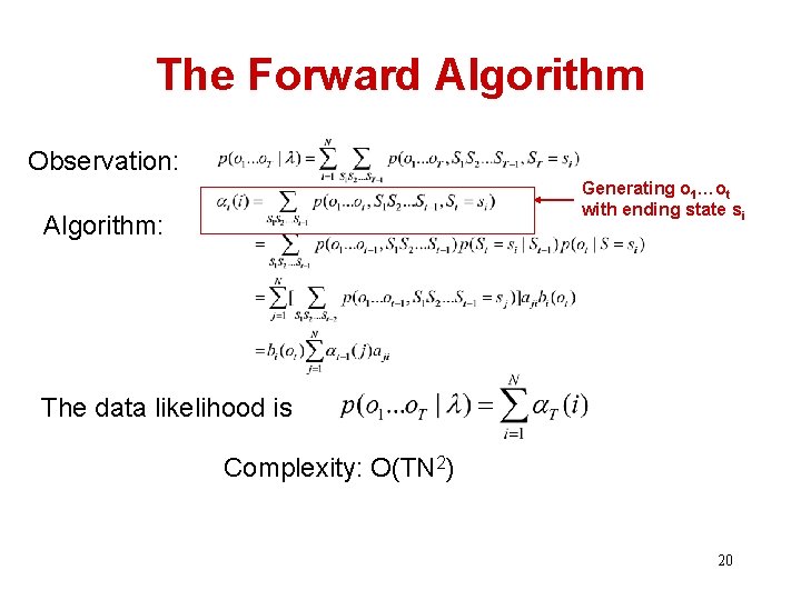
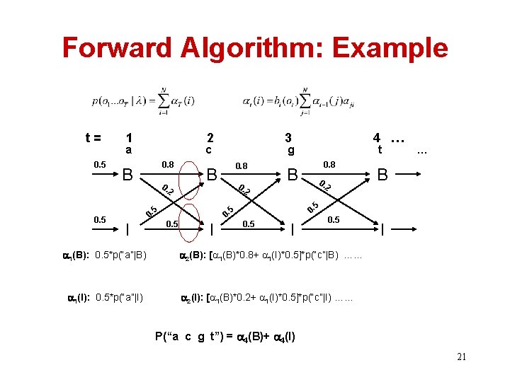
The Forward Algorithm Observation: Generating o 1…ot with ending state si Algorithm: The data likelihood is Complexity: O(TN 2) 20

Forward Algorithm: Example t= 0. 5 1 2 a c 0. 8 B 0. 2 I 1(B): 0. 5*p(“a”|B) 1(I): 0. 5*p(“a”|I) 0. 8 0. t 0. 8 B 0. 2 2 I … B 5 0. 0. 5 4 … g B 5 0. 5 3 0. 5 I 2(B): [ 1(B)*0. 8+ 1(I)*0. 5]*p(“c”|B) …… 2(I): [ 1(B)*0. 2+ 1(I)*0. 5]*p(“c”|I) …… P(“a c g t”) = 4(B)+ 4(I) 21

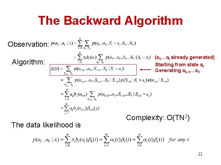
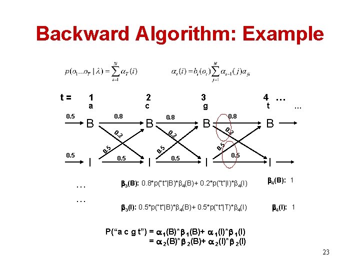
The Backward Algorithm Observation: Algorithm: The data likelihood is (o 1…ot already generated) Starting from state si Generating ot+1…o. T Complexity: O(TN 2) 22

Backward Algorithm: Example t= 0. 5 1 2 a c 0. 8 B 0. 2 … … 0. 8 0. t 0. 8 B 0. 2 2 I B 5 0. 0. 5 … 0. 5 5 I 4 … g B 0. 5 3 0. 5 I 3(B): 0. 8*p(“t”|B)* 4(B)+ 0. 2*p(“t”|I)* 4(I) 4(B): 1 3(I): 0. 5*p(“t”|B)* 4(B)+ 0. 5*p(“t”|T)* 4(I): 1 P(“a c g t”) = 1(B)* 1(B)+ 1(I)* 1(I) = 2(B)* 2(B)+ 2(I)* 2(I) 23

Problem III: Training Estimating Parameters Where do we get the probability values for all parameters? Supervised vs. Unsupervised 24

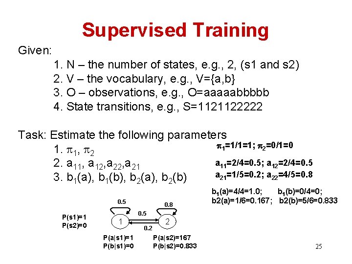
Supervised Training Given: 1. N – the number of states, e. g. , 2, (s 1 and s 2) 2. V – the vocabulary, e. g. , V={a, b} 3. O – observations, e. g. , O=aaaaabbbbb 4. State transitions, e. g. , S=1121122222 Task: Estimate the following parameters 1=1/1=1; 2=0/1=0 1. 1, 2 a 11=2/4=0. 5; a 12=2/4=0. 5 2. a 11, a 12, a 21=1/5=0. 2; a 22=4/5=0. 8 3. b 1(a), b 1(b), b 2(a), b 2(b) 0. 5 P(s 1)=1 P(s 2)=0 0. 8 b 1(a)=4/4=1. 0; b 1(b)=0/4=0; b 2(a)=1/6=0. 167; b 2(b)=5/6=0. 833 0. 5 1 P(a|s 1)=1 P(b|s 1)=0 0. 2 2 P(a|s 2)=167 P(b|s 2)=0. 833 25

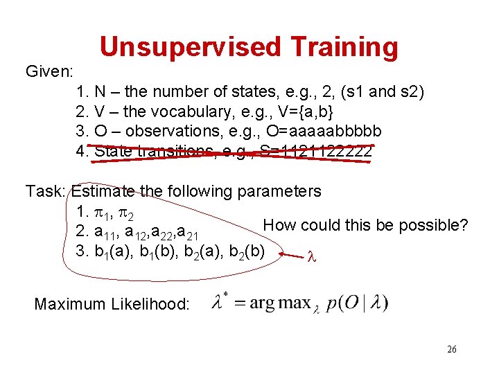
Given: Unsupervised Training 1. N – the number of states, e. g. , 2, (s 1 and s 2) 2. V – the vocabulary, e. g. , V={a, b} 3. O – observations, e. g. , O=aaaaabbbbb 4. State transitions, e. g. , S=1121122222 Task: Estimate the following parameters 1. 1, 2 How could this be possible? 2. a 11, a 12, a 21 3. b 1(a), b 1(b), b 2(a), b 2(b) Maximum Likelihood: 26

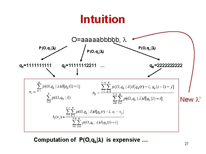
Intuition O=aaaaabbbbb, P(O, q 1| ) q 1=11111 P(O, q 2| ) P(O, q. K| ) q 2=11111112211 … q. K=22222 New ’ Computation of P(O, qk| ) is expensive … 27

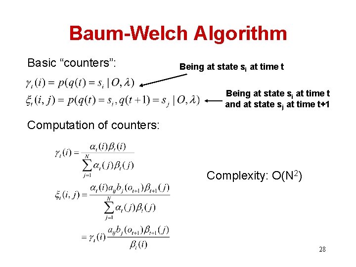
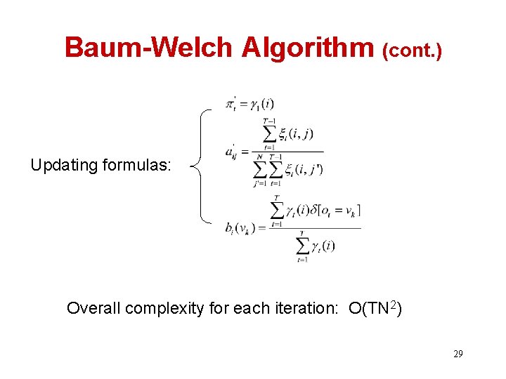
Baum-Welch Algorithm Basic “counters”: Being at state si at time t and at state sj at time t+1 Computation of counters: Complexity: O(N 2) 28

Baum-Welch Algorithm (cont. ) Updating formulas: Overall complexity for each iteration: O(TN 2) 29

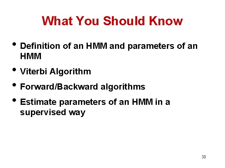
What You Should Know • Definition of an HMM and parameters of an HMM • Viterbi Algorithm • Forward/Backward algorithms • Estimate parameters of an HMM in a supervised way 30