Clusters in data Common Statistical Task Find Clusters

Clusters in data Common Statistical Task: Find Clusters in Data • Interesting sub-populations? • Important structure in data? • How to do this? PCA & visualization is very simple approach There is a large literature of other methods (will study more later)

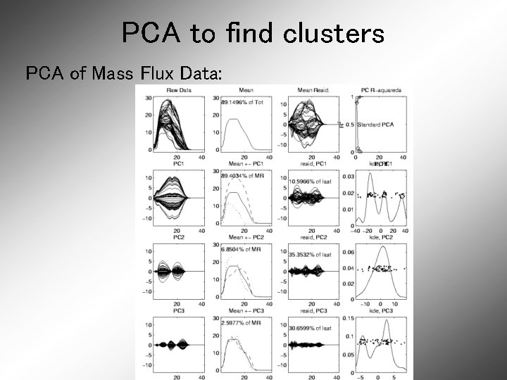
PCA to find clusters PCA of Mass Flux Data:

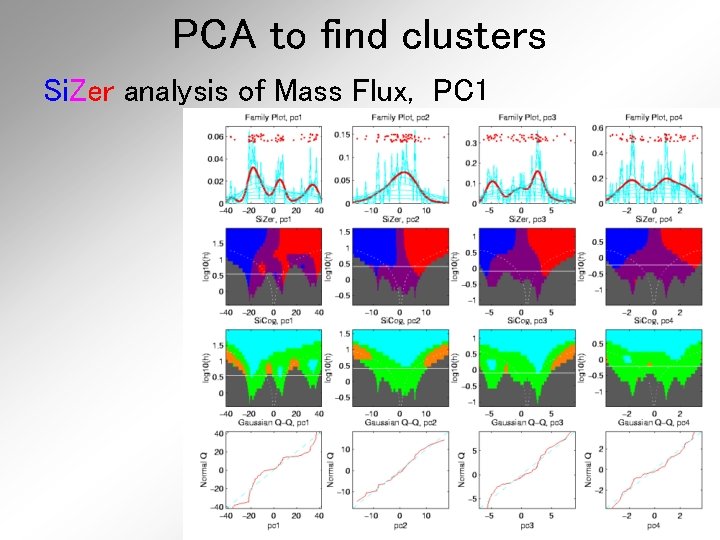
PCA to find clusters Return to Investigation of PC 1 Clusters: • Can see 3 bumps in smooth histogram Main Question: Important structure or OODA: sampling variability? Confirmatory Analysis Approach: Si. Zer (SIgnificance of ZERo crossings of deriv. )

Statistical Smoothing In 1 Dimension, 2 Major Settings: • Density Estimation “Histograms” • Nonparametric Regression “Scatterplot Smoothing”

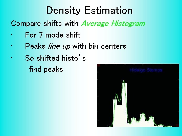
Density Estimation Compare shifts with Average Histogram • For 7 mode shift • Peaks line up with bin centers • So shifted histo’s find peaks

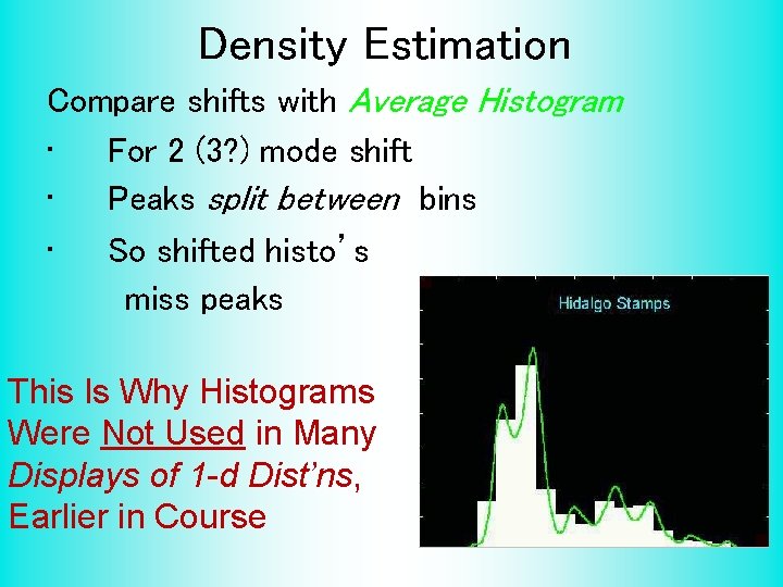
Density Estimation Compare shifts with Average Histogram • For 2 (3? ) mode shift • Peaks split between bins • So shifted histo’s miss peaks This Is Why Histograms Were Not Used in Many Displays of 1 -d Dist’ns, Earlier in Course

Density Estimation Histogram Drawbacks: • Need to choose bin width • Need to choose bin location • But Average Histogram reveals structure • So should use that, instead of histo Name: Kernel Density Estimate

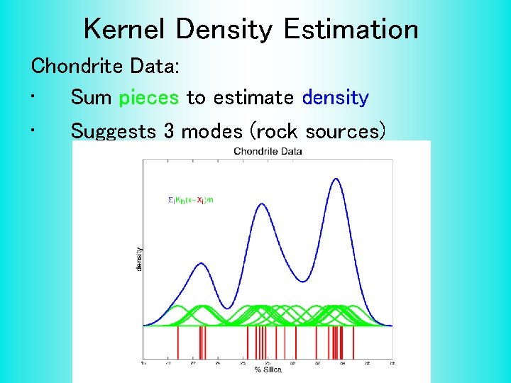
Kernel Density Estimation Chondrite Data: • Sum pieces to estimate density • Suggests 3 modes (rock sources)

Statistical Smoothing 2 Major Settings: • Density Estimation “Histograms” • Nonparametric Regression “Scatterplot Smoothing”

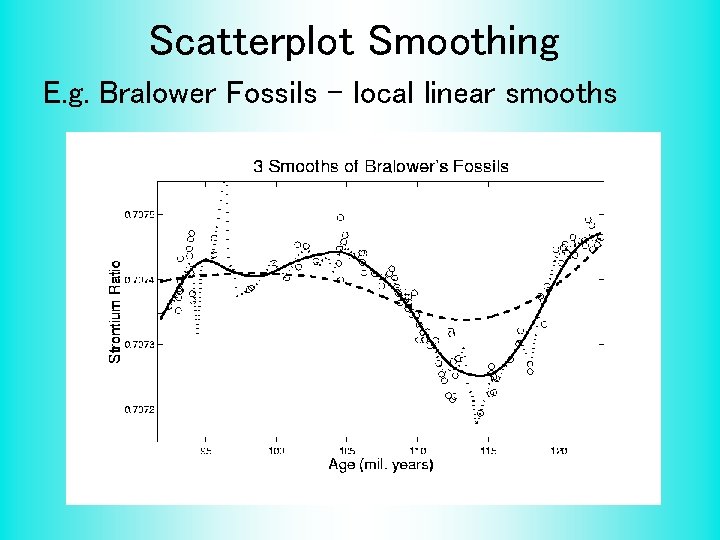
Scatterplot Smoothing E. g. Bralower Fossils – local linear smooths

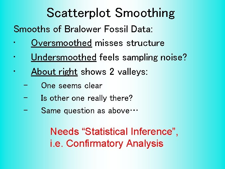
Scatterplot Smoothing Smooths of Bralower Fossil Data: • Oversmoothed misses structure • Undersmoothed feels sampling noise? • About right shows 2 valleys: – – – One seems clear Is other one really there? Same question as above… Needs “Statistical Inference”, i. e. Confirmatory Analysis

Si. Zer Background Scale Space – Idea from Computer Vision Goal: Teach Computers to “See” Modern Research: Extract “Information” from Images Early Theoretical work

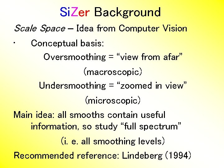
Si. Zer Background Scale Space – Idea from Computer Vision • Conceptual basis: Oversmoothing = “view from afar” (macroscopic) Undersmoothing = “zoomed in view” (microscopic) Main idea: all smooths contain useful information, so study “full spectrum” (i. e. all smoothing levels) Recommended reference: Lindeberg (1994)

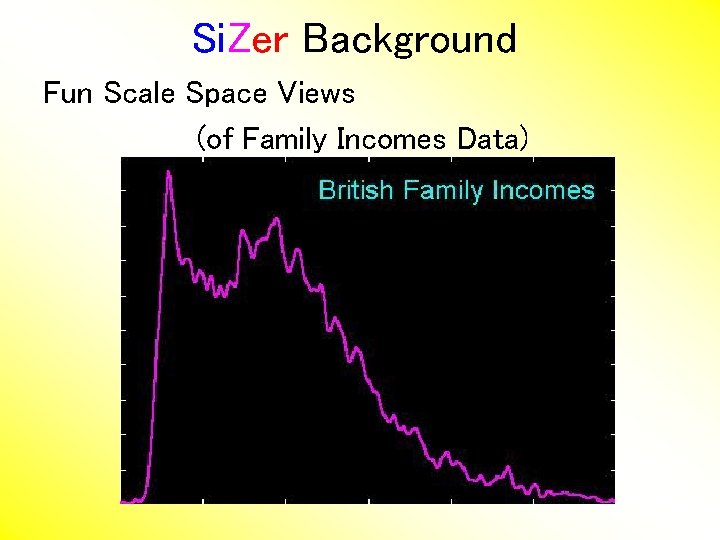
Si. Zer Background Fun Scale Space Views (of Family Incomes Data)

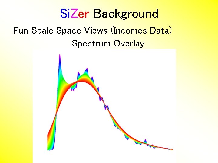
Si. Zer Background Fun Scale Space Views (Incomes Data) Spectrum Overlay

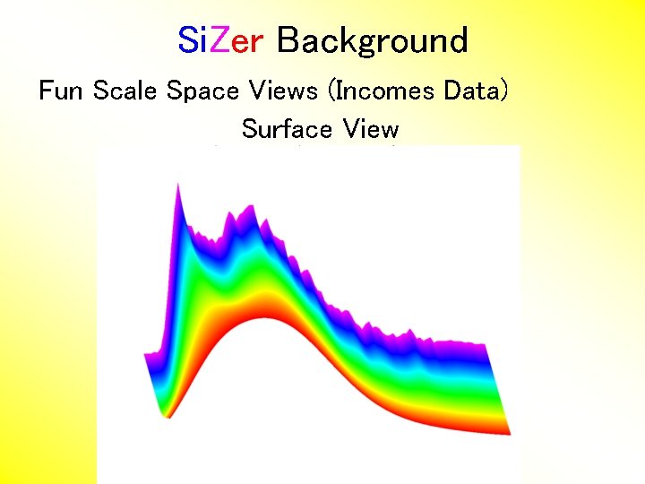
Si. Zer Background Fun Scale Space Views (Incomes Data) Surface View

Si. Zer Background Fun Scale Space Views (of Family Incomes Data) Note: The scale space viewpoint makes Data Dased Bandwidth Selection Much less important (than I once thought…. )

Si. Zer Background Si. Zer: • Significance of Zero crossings, of the derivative, in scale space • Combines: – – • • needed statistical inference novel visualization To get: a powerful exploratory data analysis method Main references: Chaudhuri & Marron (1999) Hannig & Marron (2006)

Si. Zer Background Basic idea: a bump is characterized by: • an increase • followed by a decrease Generalization: Many features of interest captured by sign of the slope of the smooth Foundation of Si. Zer: Statistical inference on slopes, over scale space

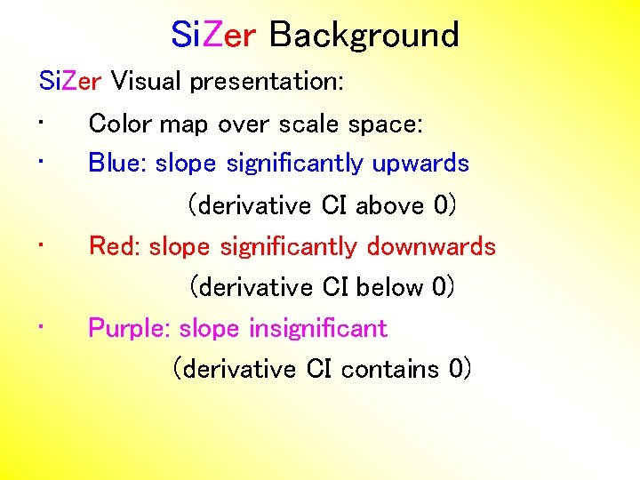
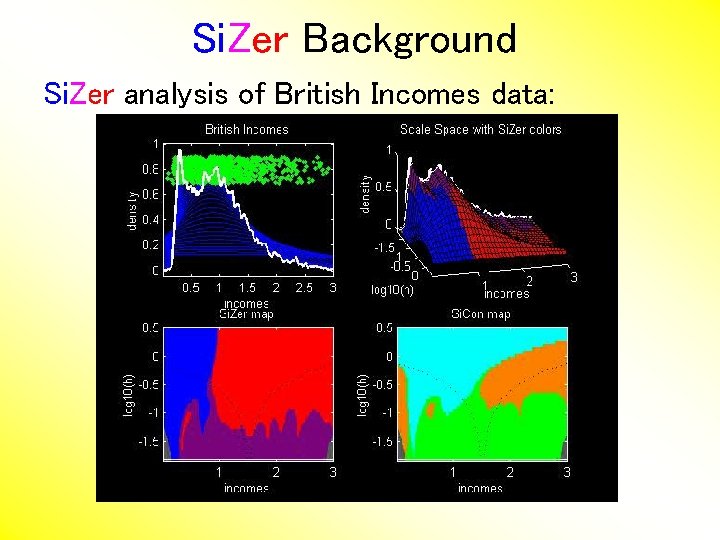
Si. Zer Background Si. Zer Visual presentation: • Color map over scale space: • Blue: slope significantly upwards (derivative CI above 0) • Red: slope significantly downwards (derivative CI below 0) • Purple: slope insignificant (derivative CI contains 0)

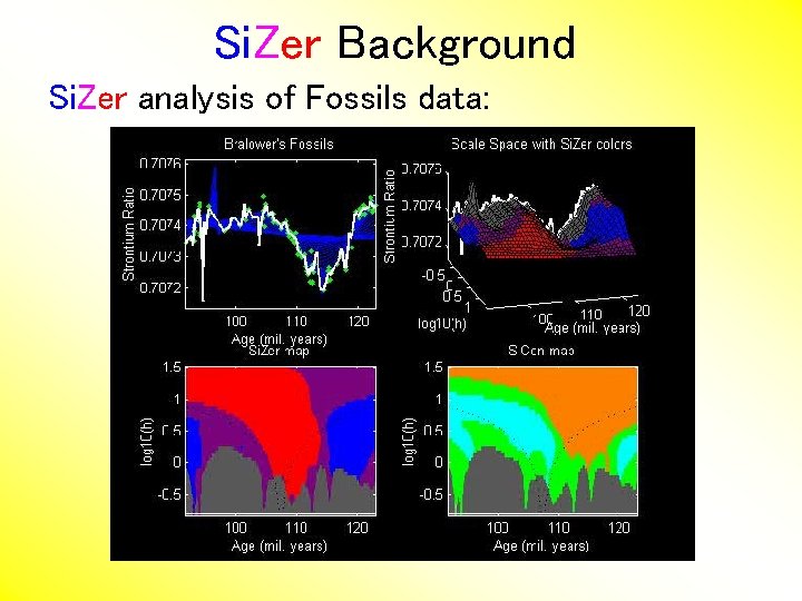
Si. Zer Background Si. Zer analysis of Fossils data:

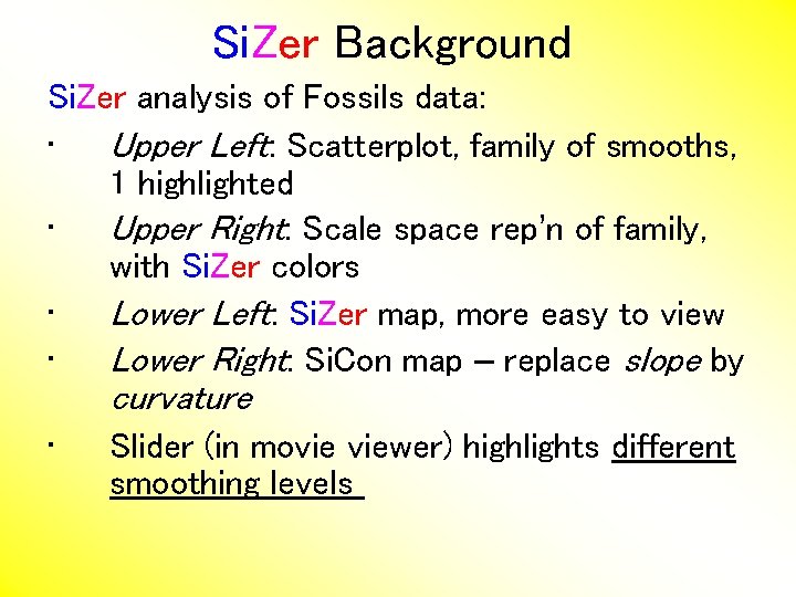
Si. Zer Background Si. Zer analysis of Fossils data: • Upper Left: Scatterplot, family of smooths, 1 highlighted • Upper Right: Scale space rep’n of family, with Si. Zer colors • Lower Left: Si. Zer map, more easy to view • Lower Right: Si. Con map – replace slope by curvature • Slider (in movie viewer) highlights different smoothing levels

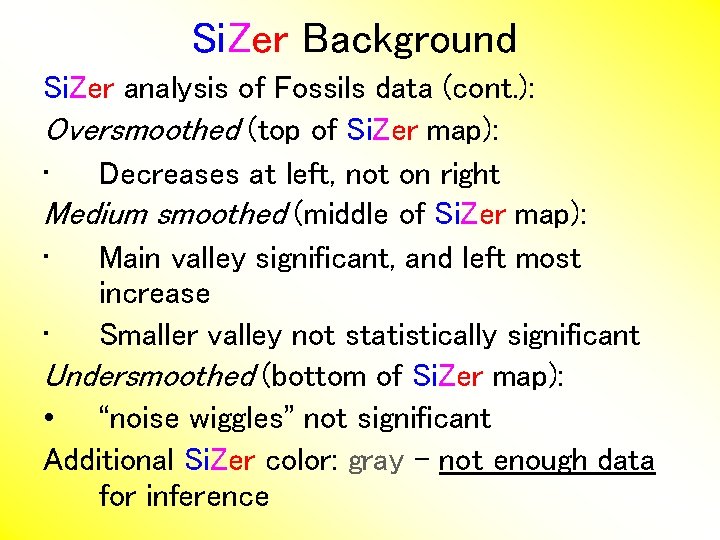
Si. Zer Background Si. Zer analysis of Fossils data (cont. ): Oversmoothed (top of Si. Zer map): • Decreases at left, not on right Medium smoothed (middle of Si. Zer map): • Main valley significant, and left most increase • Smaller valley not statistically significant Undersmoothed (bottom of Si. Zer map): • “noise wiggles” not significant Additional Si. Zer color: gray - not enough data for inference

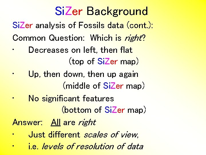
Si. Zer Background Si. Zer analysis of Fossils data (cont. ): Common Question: Which is right? • Decreases on left, then flat (top of Si. Zer map) • Up, then down, then up again (middle of Si. Zer map) • No significant features (bottom of Si. Zer map) Answer: All are right • Just different scales of view, • i. e. levels of resolution of data

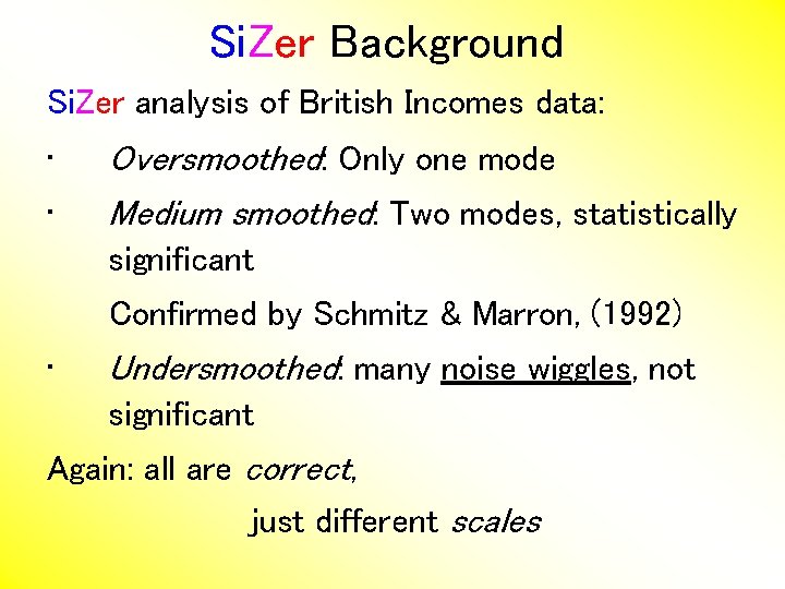
Si. Zer Background Si. Zer analysis of British Incomes data:

Si. Zer Background Si. Zer analysis of British Incomes data: • • Oversmoothed: Only one mode Medium smoothed: Two modes, statistically significant Confirmed by Schmitz & Marron, (1992) • Undersmoothed: many noise wiggles, not significant Again: all are correct, just different scales

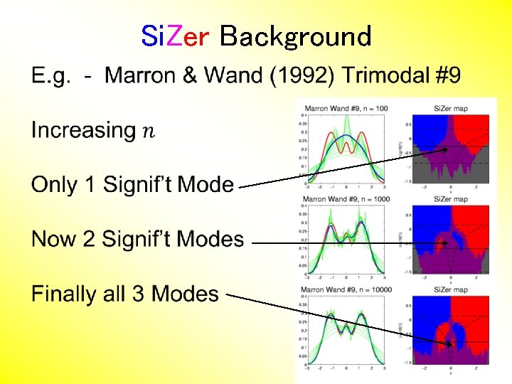
Si. Zer Background •

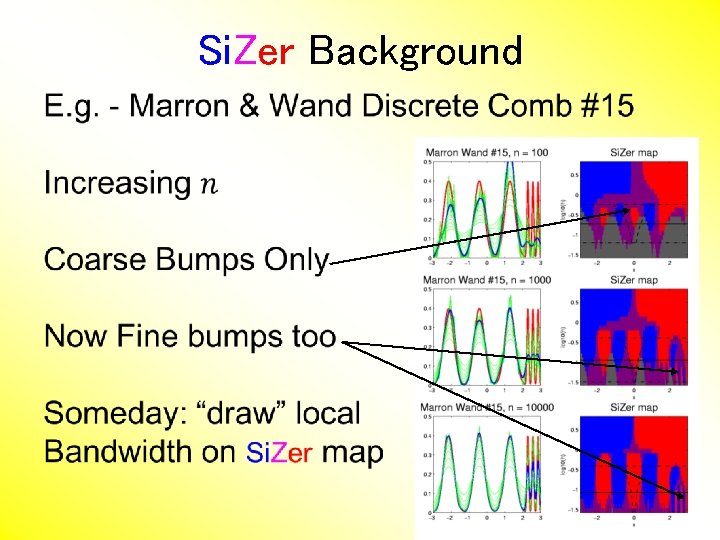
Si. Zer Background •

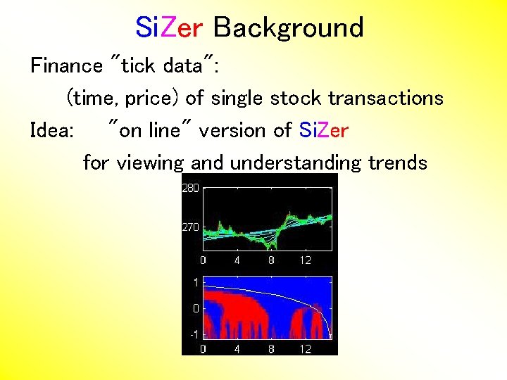
Si. Zer Background Finance "tick data": (time, price) of single stock transactions Idea: "on line" version of Si. Zer for viewing and understanding trends

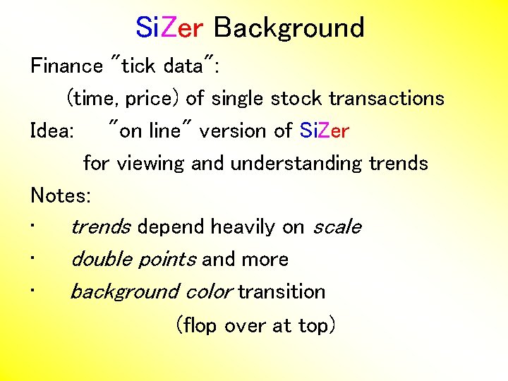
Si. Zer Background Finance "tick data": (time, price) of single stock transactions Idea: "on line" version of Si. Zer for viewing and understanding trends Notes: • trends depend heavily on scale • double points and more • background color transition (flop over at top)

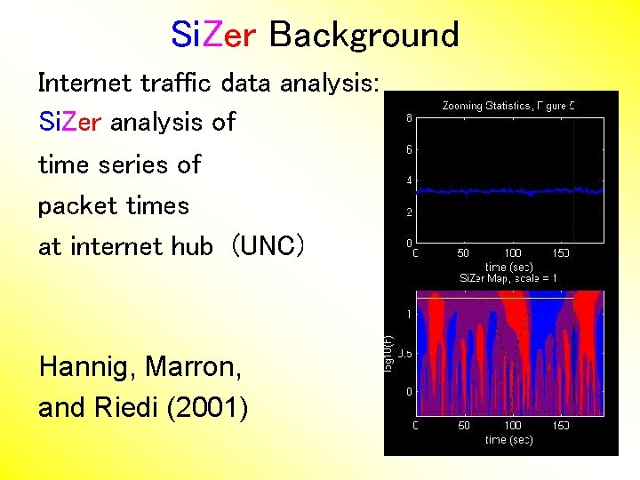
Si. Zer Background Internet traffic data analysis: Si. Zer analysis of time series of packet times at internet hub (UNC) Hannig, Marron, and Riedi (2001)

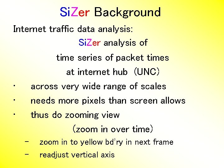
Si. Zer Background Internet traffic data analysis: Si. Zer analysis of time series of packet times at internet hub (UNC) • across very wide range of scales • needs more pixels than screen allows • thus do zooming view (zoom in over time) – – zoom in to yellow bd’ry in next frame readjust vertical axis

Si. Zer Background Internet traffic data analysis (cont. ) Insights from Si. Zer analysis: • Coarse scales: amazing amount of significant structure • Evidence of self-similar fractal type process? • Fewer significant features at small scales • But they exist, so not Poisson process • • Poisson approximation OK at small scale? ? ? Smooths (top part) stable at large scales?

Dependent Si. Zer Rondonotti, Marron, and Park (2007) • Si. Zer compares data with white noise • Inappropriate in time series • Dependent Si. Zer compares data with an assumed model • Visual Goodness of Fit test

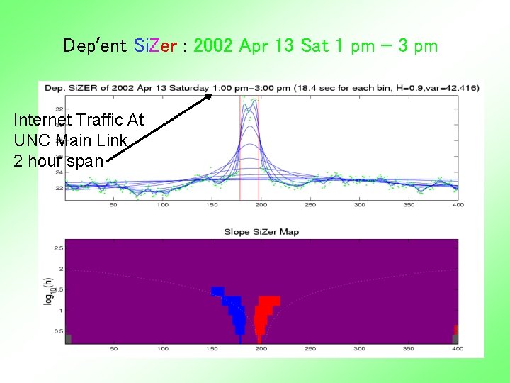
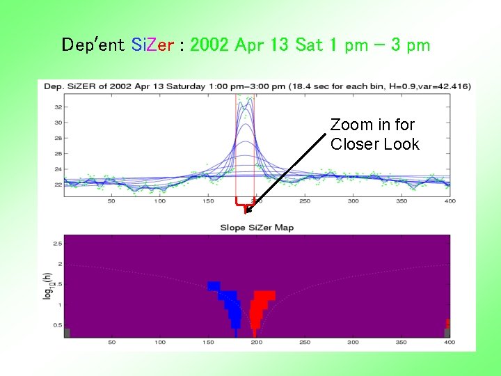
Dep’ent Si. Zer : 2002 Apr 13 Sat 1 pm – 3 pm Internet Traffic At UNC Main Link 2 hour span

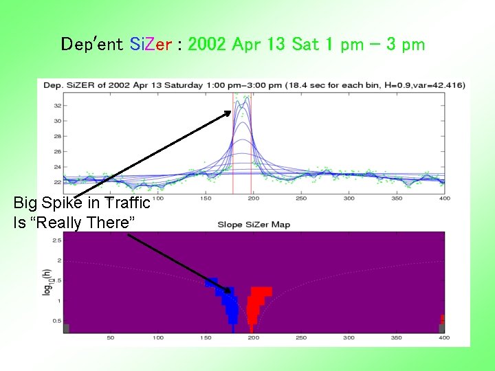
Dep’ent Si. Zer : 2002 Apr 13 Sat 1 pm – 3 pm Big Spike in Traffic Is “Really There”

Dep’ent Si. Zer : 2002 Apr 13 Sat 1 pm – 3 pm Zoom in for Closer Look

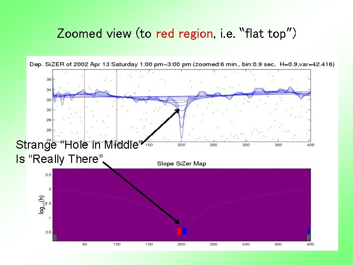
Zoomed view (to red region, i. e. “flat top”) Strange “Hole in Middle” Is “Really There”

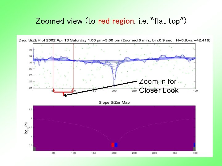
Zoomed view (to red region, i. e. “flat top”) Zoom in for Closer Look

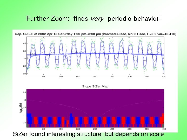
Further Zoom: finds very periodic behavior! Si. Zer found interesting structure, but depends on scale

Possible Physical Explanation IP “Port Scan” • Common device of hackers • Searching for “break in points” • Send query to every possible (within UNC domain): – IP address – Port Number • Replies can indicate system weaknesses Internet Traffic is hard to model

Si. Zer Background Historical Note & Acknowledgements: Scale Space: Si. Zer: S. M. Pizer Probal Chaudhuri Main References: Chaudhuri & Marron (1999) Chaudhuri & Marron (2000) Hannig & Marron (2006)

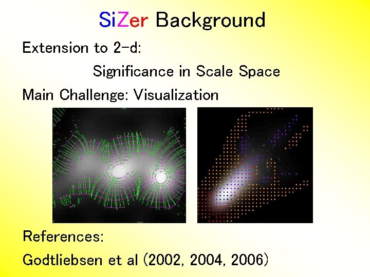
Si. Zer Background Extension to 2 -d: Significance in Scale Space Main Challenge: Visualization References: Godtliebsen et al (2002, 2004, 2006)

Si. Zer Overview Would you like to try smoothing & Si. Zer? • Marron Software Website as Before • In “Smoothing” Directory: • – kde. SM. m – npr. SM. m – sizer. SM. m Recall: “>> help sizer. SM” for usage

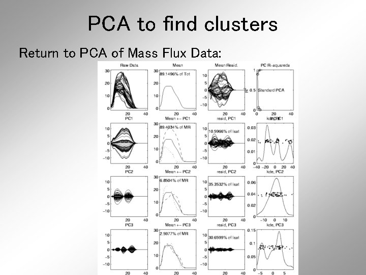
PCA to find clusters Return to PCA of Mass Flux Data:

PCA to find clusters Si. Zer analysis of Mass Flux, PC 1

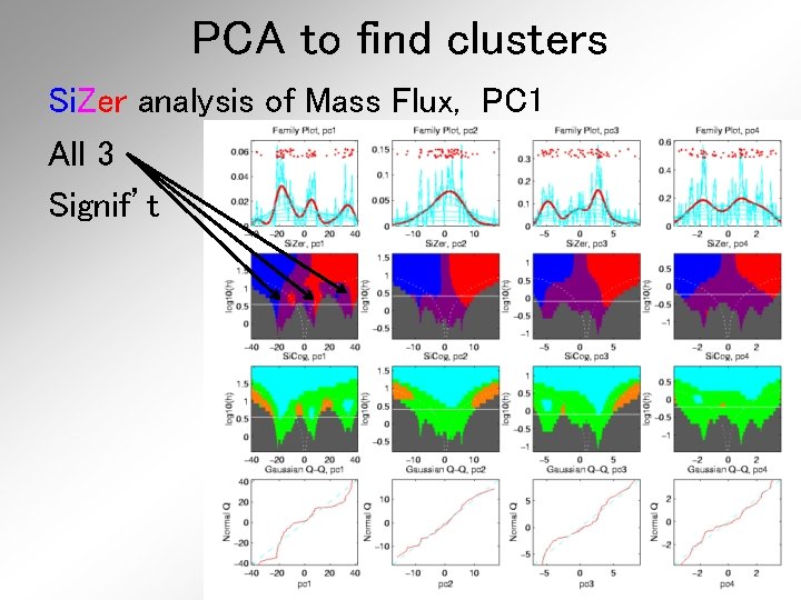
PCA to find clusters Si. Zer analysis of Mass Flux, PC 1 All 3 Signif’t

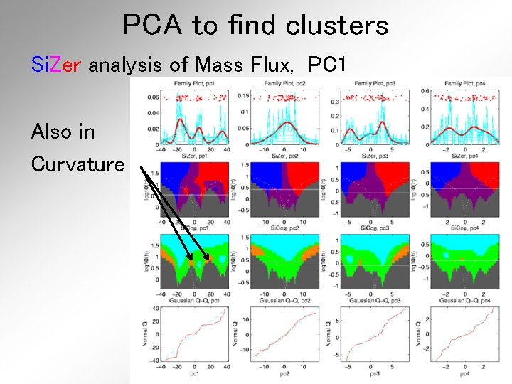
PCA to find clusters Si. Zer analysis of Mass Flux, PC 1 Also in Curvature

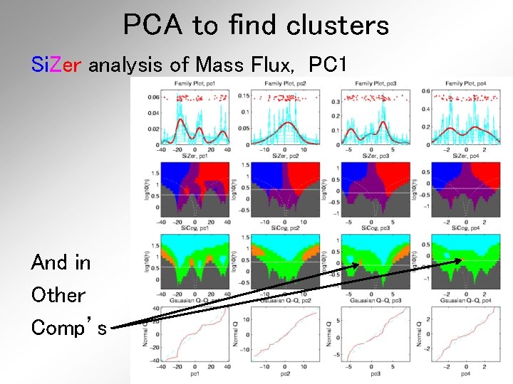
PCA to find clusters Si. Zer analysis of Mass Flux, PC 1 And in Other Comp’s

PCA to find clusters Si. Zer analysis of Mass Flux, PC 1 Conclusion: • Found 3 significant clusters! • Worth deeper investigation • Correspond to 3 known “cloud types”

Recall Yeast Cell Cycle Data • “Gene Expression” – Micro-array data • Data (after major preprocessing): Expression “level” of: • thousands of genes (d ~ 1, 000 s) • but only dozens of “cases” (n ~ 10 s) • Interesting statistical issue: High Dimension Low Sample Size data (HDLSS)

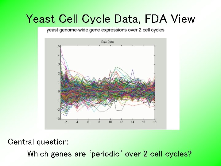
Yeast Cell Cycle Data, FDA View Central question: Which genes are “periodic” over 2 cell cycles?

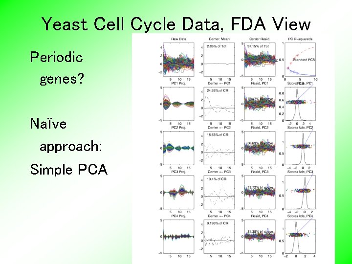
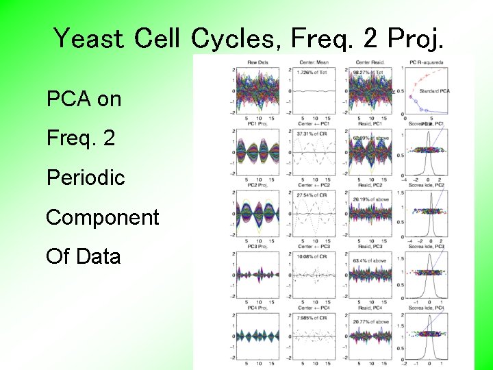
Yeast Cell Cycle Data, FDA View Periodic genes? Naïve approach: Simple PCA

Yeast Cell Cycles, Freq. 2 Proj. PCA on Freq. 2 Periodic Component Of Data

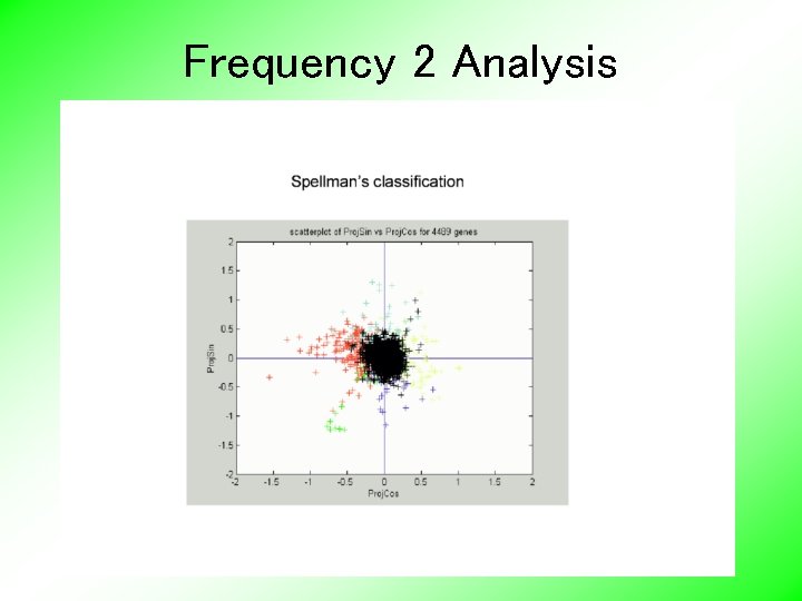
Frequency 2 Analysis • Project data onto 2 -dim space of sin and cos (freq. 2) • Useful view: scatterplot • Angle (in polar coordinates) shows phase Approach from Zhao, Marron & Wells (2004)

Frequency 2 Analysis

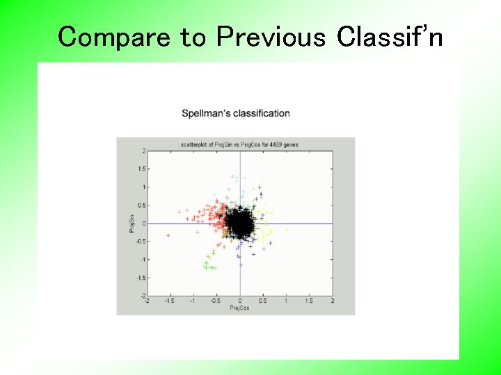
Frequency 2 Analysis • Project data onto 2 -dim space of sin and cos (freq. 2) • Useful view: scatterplot • • Angle (in polar coordinates) shows phase Colors: Spellman’s cell cycle phase classification • Black was labeled “not periodic” • Within class phases approx’ly same, but notable differences Now try to improve “phase classification” •

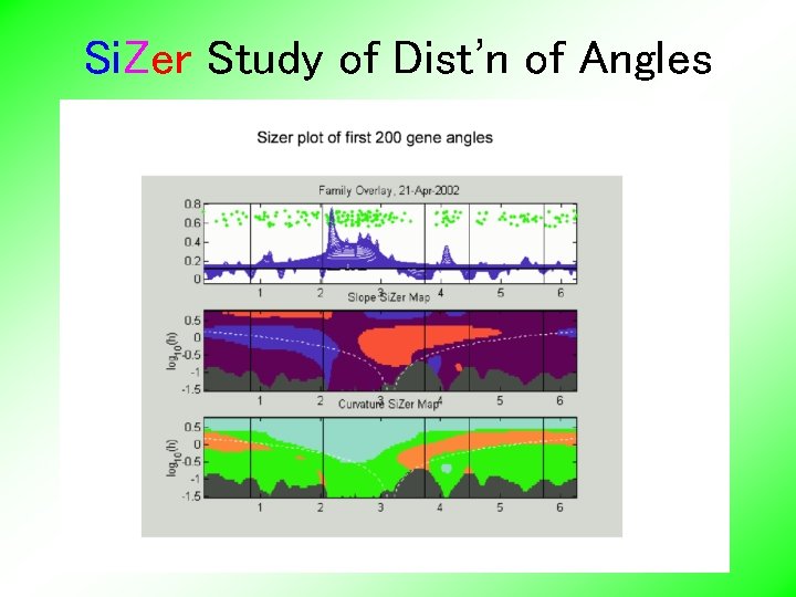
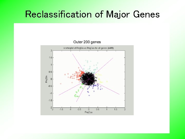
Yeast Cell Cycle Revisit “phase classification”, • • • approach: Use outer 200 genes (other numbers tried, less resolution) Study distribution of angles Use Si. Zer analysis (finds significant bumps, etc. , in histogram) Carefully redrew boundaries Check by studying k. d. e. angles

Si. Zer Study of Dist’n of Angles

Reclassification of Major Genes

Compare to Previous Classif’n

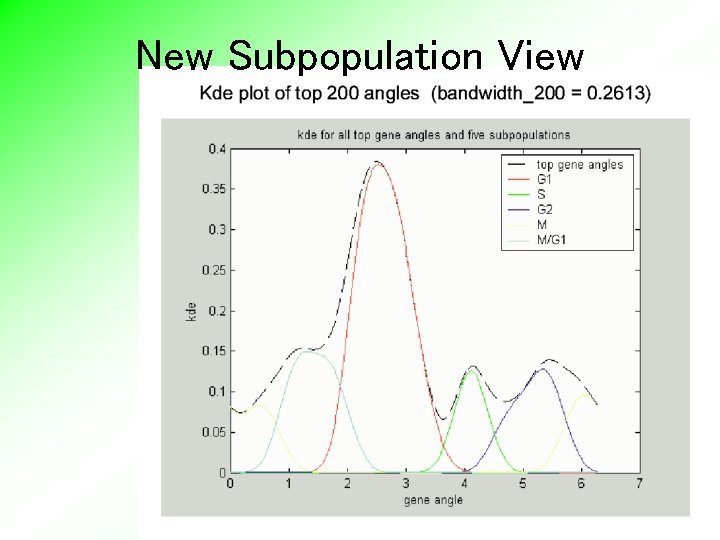
New Subpopulation View

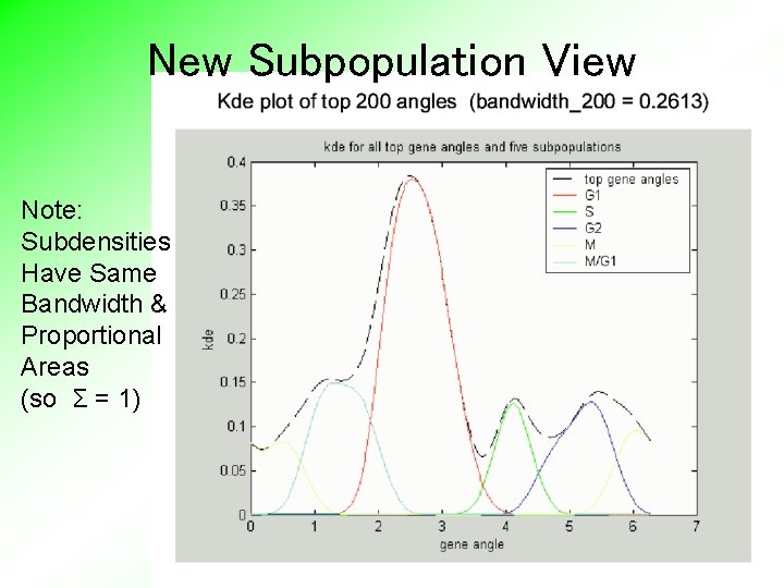
New Subpopulation View Note: Subdensities Have Same Bandwidth & Proportional Areas (so Σ = 1)

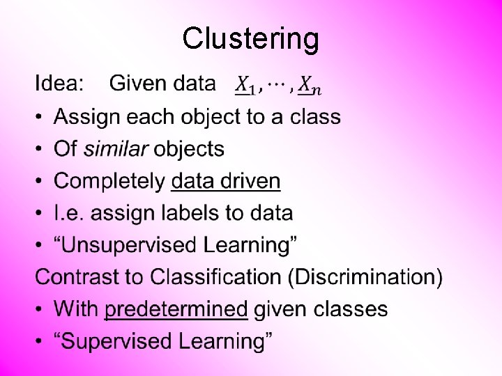
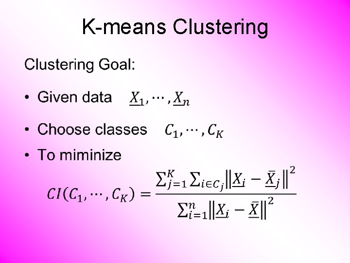
Clustering •

Clustering Important References: • Mac. Queen (1967) • Hartigan (1975) • Gersho and Gray (1992) • Kaufman and Rousseeuw (2005) See Also: Wikipedia

K-means Clustering •

K-means Clustering •

K-means Clustering •

K-means Clustering •

K-means Clustering •

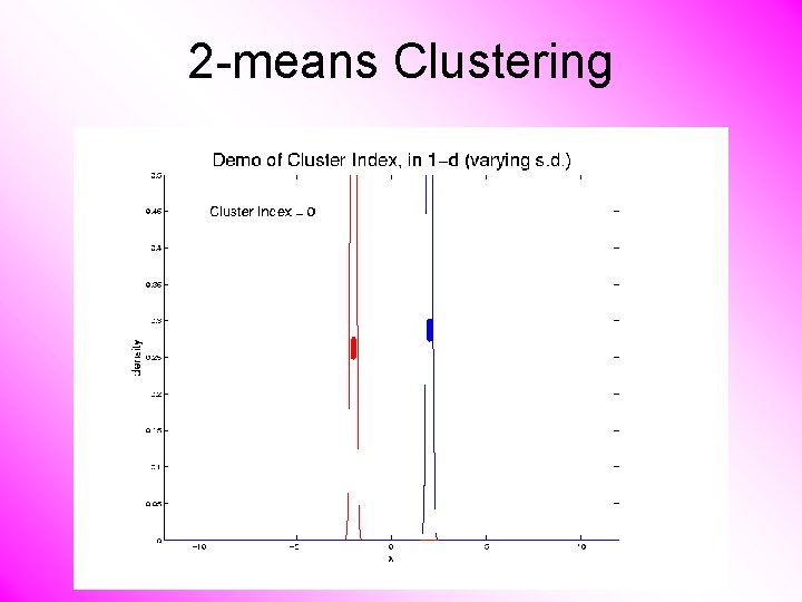
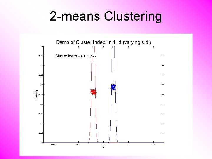
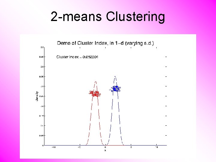
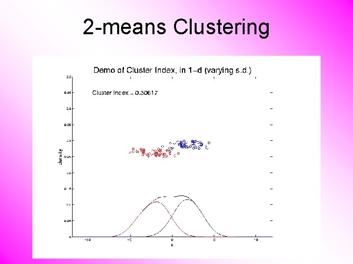
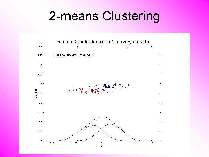
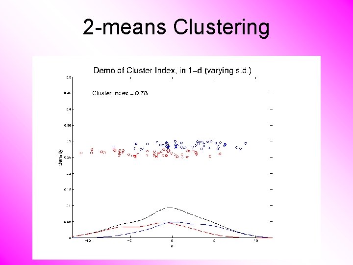
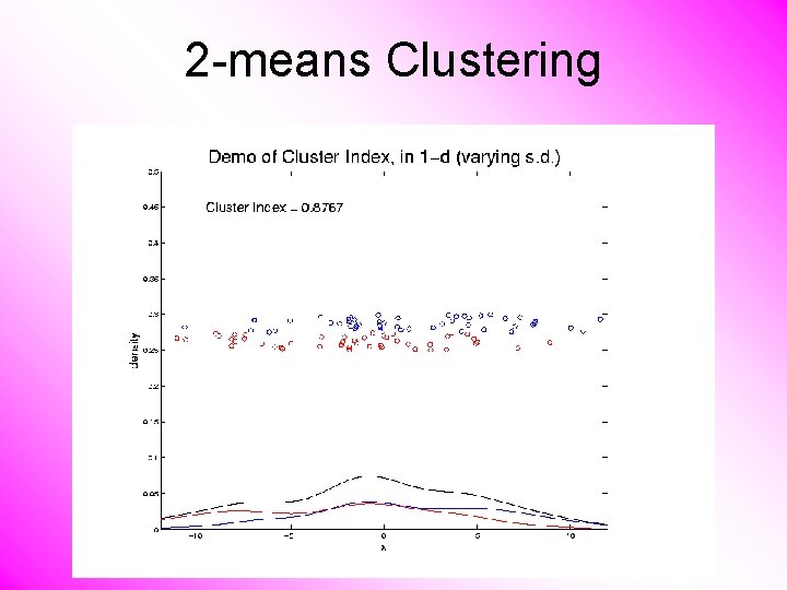
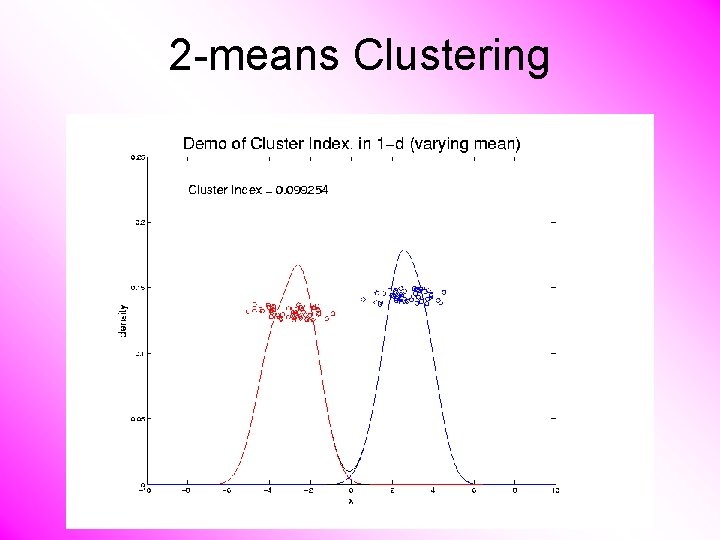
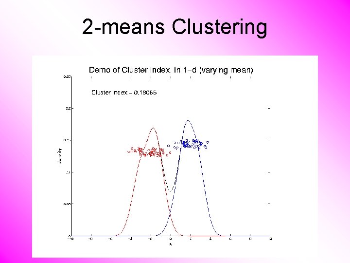
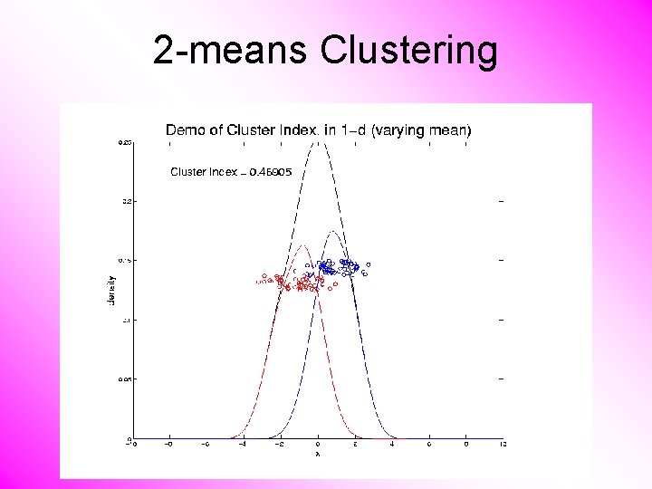
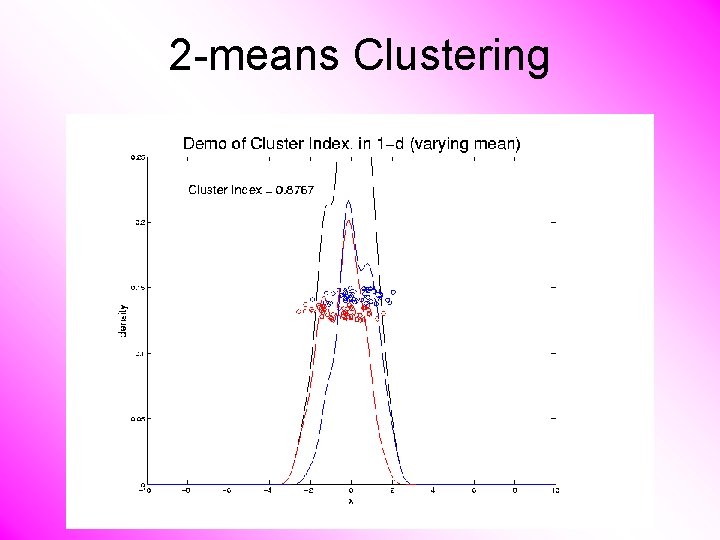
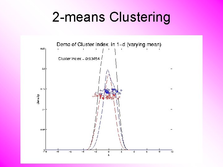
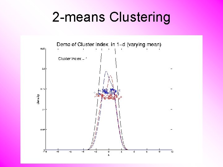
2 -means Clustering Study CI, using simple 1 -d examples • Varying Standard Deviation

2 -means Clustering

2 -means Clustering

2 -means Clustering

2 -means Clustering

2 -means Clustering

2 -means Clustering

2 -means Clustering

2 -means Clustering

2 -means Clustering

2 -means Clustering

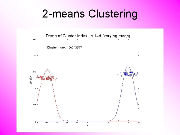
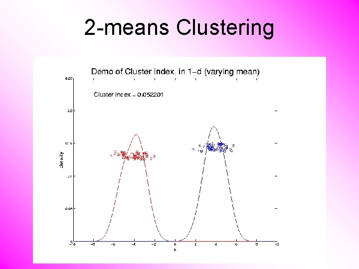
2 -means Clustering Study CI, using simple 1 -d examples • Varying Standard Deviation • Varying Mean

2 -means Clustering

2 -means Clustering

2 -means Clustering

2 -means Clustering

2 -means Clustering

2 -means Clustering

2 -means Clustering

2 -means Clustering

2 -means Clustering

2 -means Clustering

2 -means Clustering

2 -means Clustering

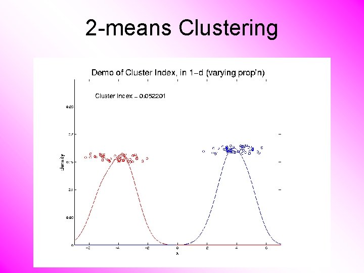
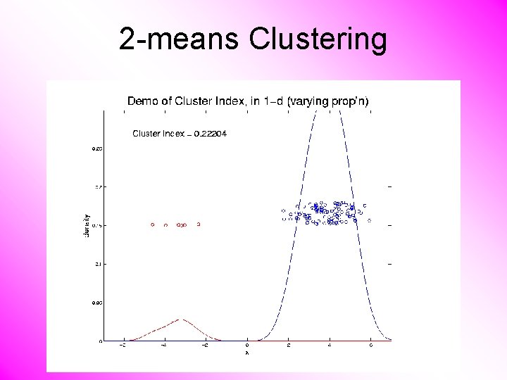
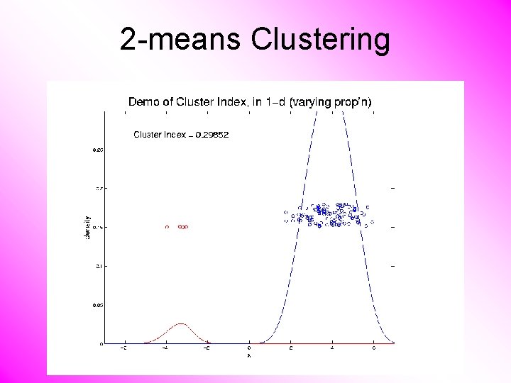
2 -means Clustering Study CI, using simple 1 -d examples • Varying Standard Deviation • Varying Mean • Varying Proportion

2 -means Clustering

2 -means Clustering

2 -means Clustering

2 -means Clustering

2 -means Clustering

2 -means Clustering

2 -means Clustering

2 -means Clustering

2 -means Clustering

2 -means Clustering

2 -means Clustering

2 -means Clustering

2 -means Clustering

2 -means Clustering

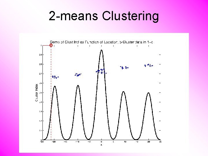
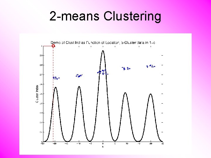
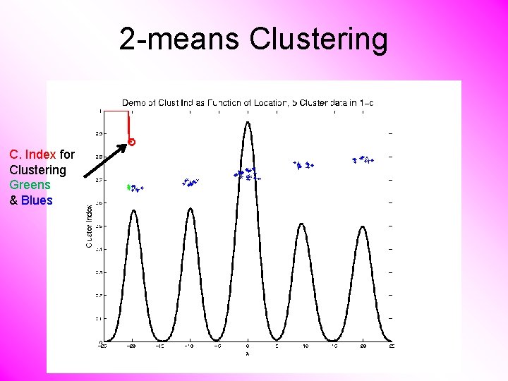
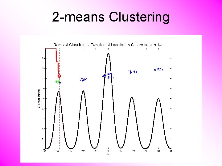
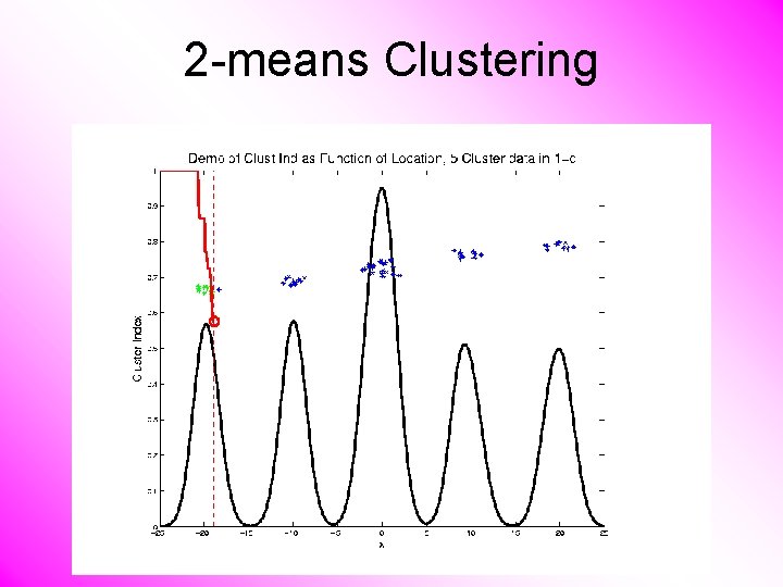
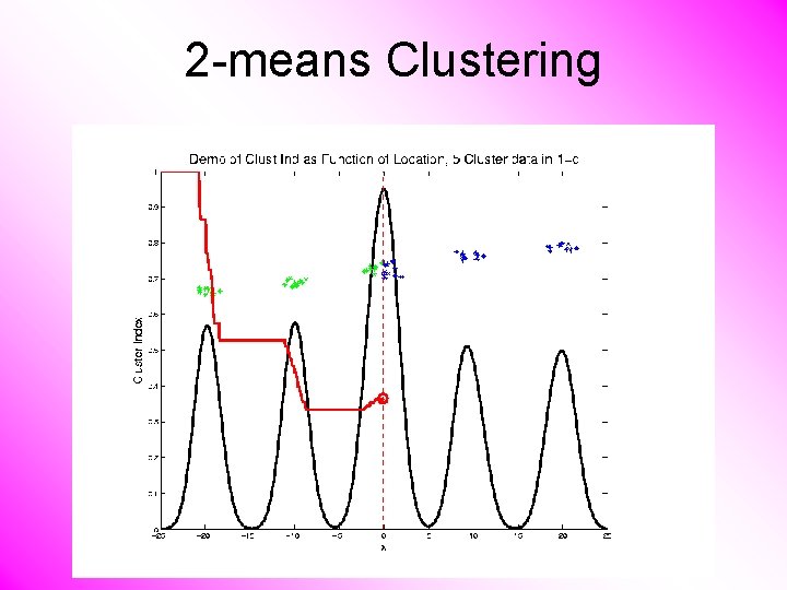
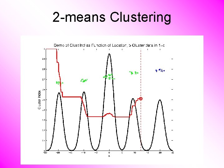
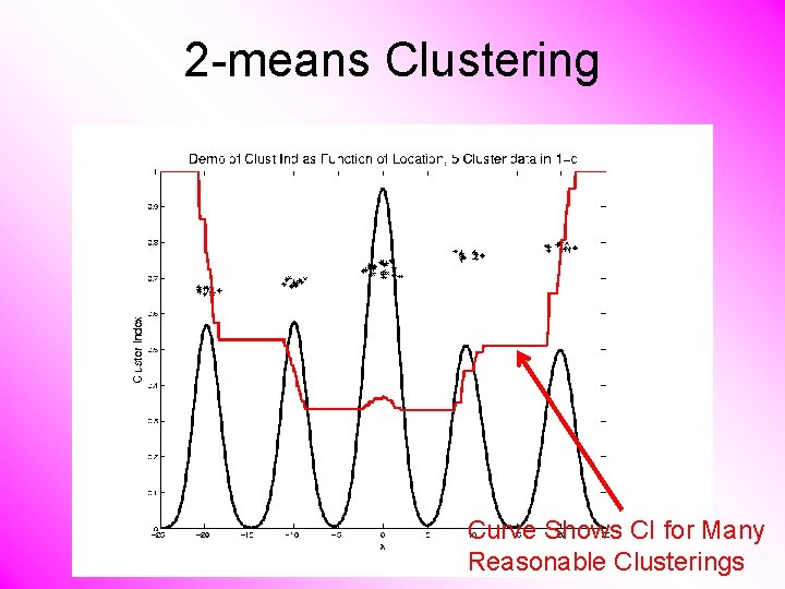
2 -means Clustering Study CI, using simple 1 -d examples • Over changing Classes (moving b’dry)

2 -means Clustering

2 -means Clustering

2 -means Clustering

2 -means Clustering C. Index for Clustering Greens & Blues

2 -means Clustering

2 -means Clustering

2 -means Clustering

2 -means Clustering

2 -means Clustering

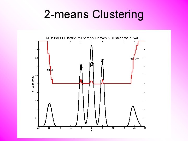
2 -means Clustering Curve Shows CI for Many Reasonable Clusterings

2 -means Clustering •

2 -means Clustering

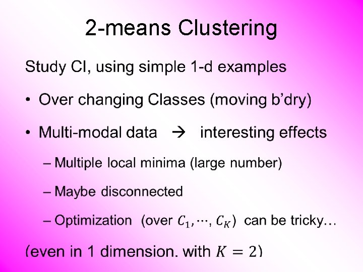
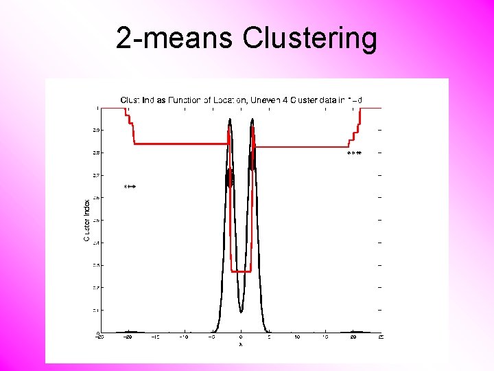
2 -means Clustering Study CI, using simple 1 -d examples • Over changing Classes (moving b’dry) • Multi-modal data interesting effects – Can have 4 (or more) local mins (even in 1 dimension, with K = 2)

2 -means Clustering

2 -means Clustering Study CI, using simple 1 -d examples • Over changing Classes (moving b’dry) • Multi-modal data interesting effects – Local mins can be hard to find – i. e. iterative procedures can “get stuck” (even in 1 dimension, with K = 2)

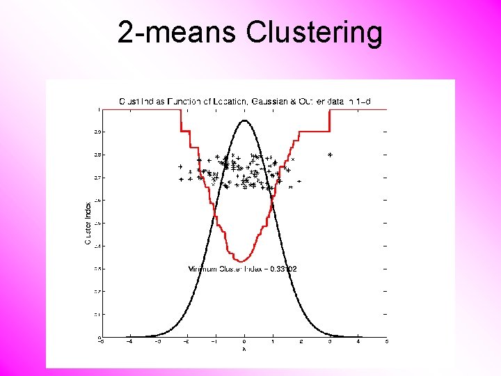
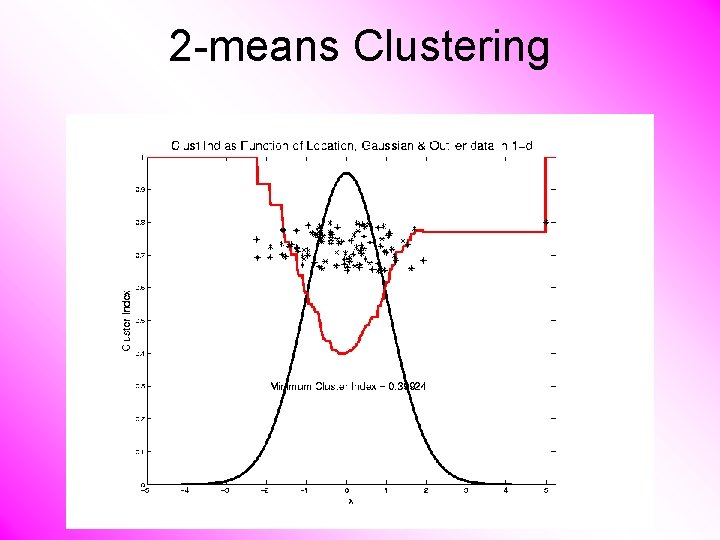
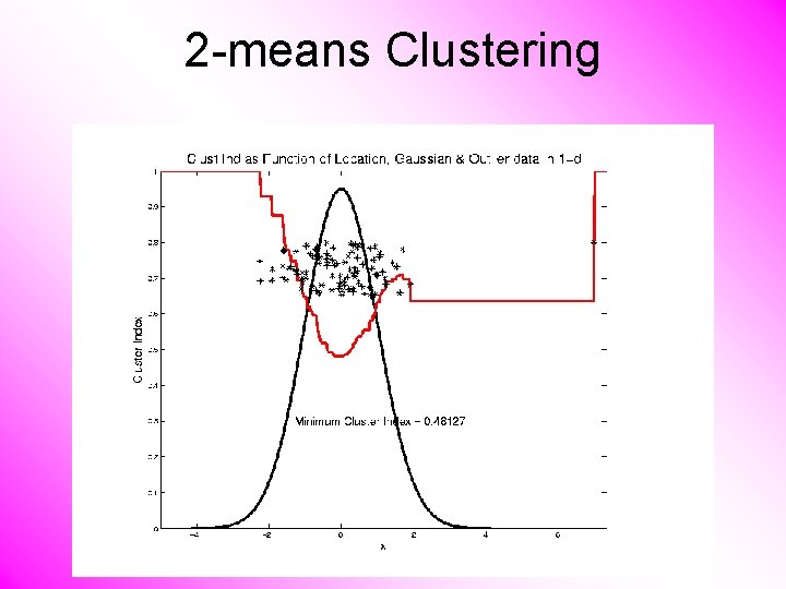
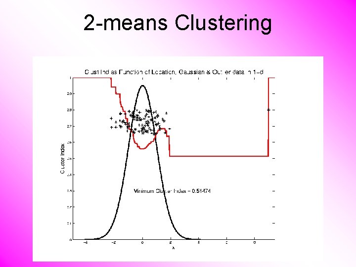
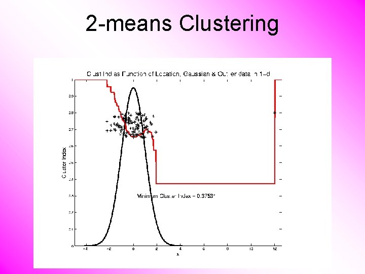
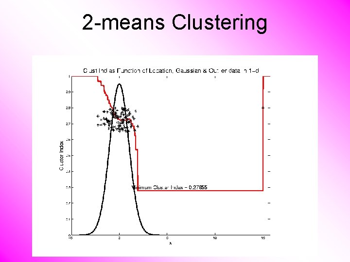
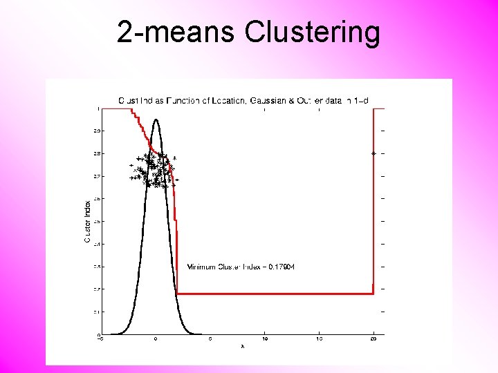
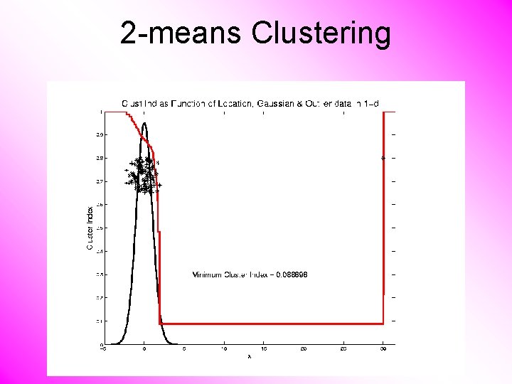
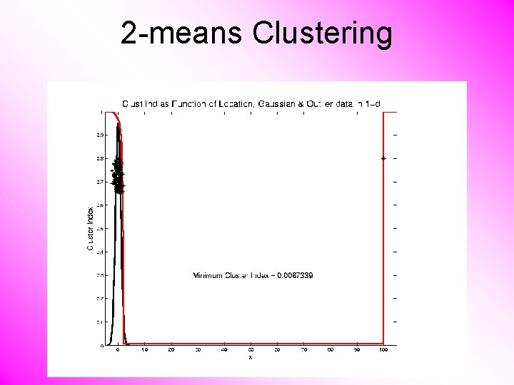
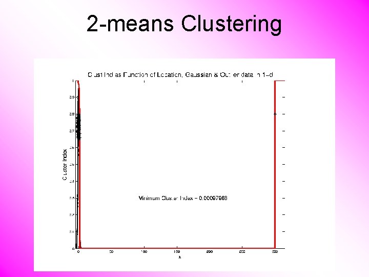
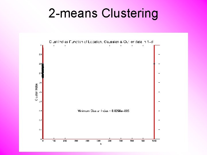
2 -means Clustering Study CI, using simple 1 -d examples • Effect of a single outlier?

2 -means Clustering

2 -means Clustering

2 -means Clustering

2 -means Clustering

2 -means Clustering

2 -means Clustering

2 -means Clustering

2 -means Clustering

2 -means Clustering

2 -means Clustering

2 -means Clustering

2 -means Clustering Study CI, using simple 1 -d examples • Effect of a single outlier? – Can create local minimum – Can also yield a global minimum – This gives a one point class – Can make CI arbitrarily small (really a “good clustering”? ? ? )

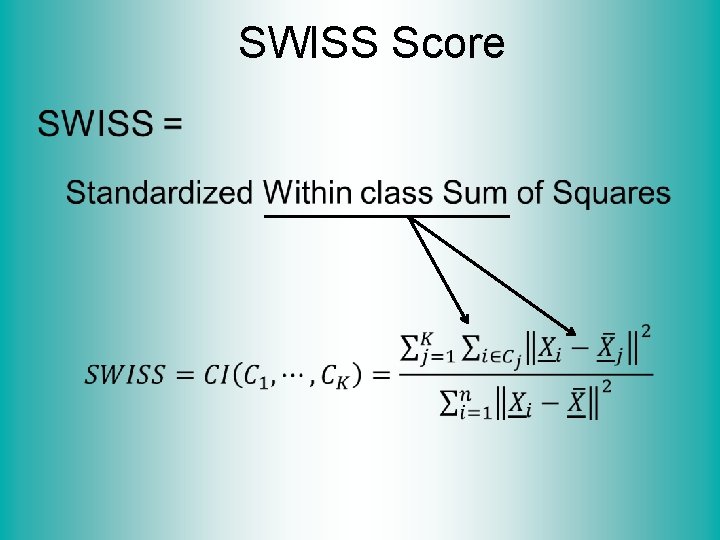
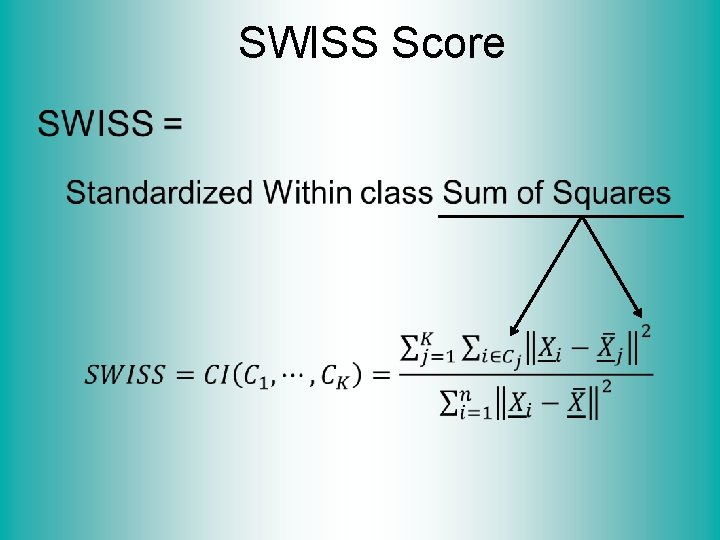
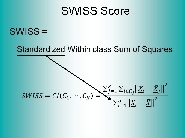
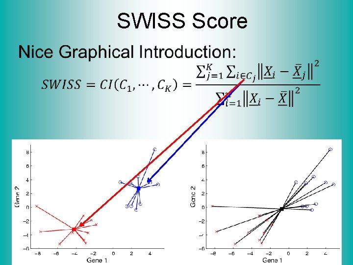
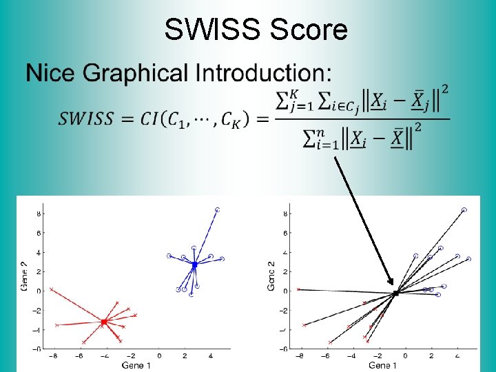
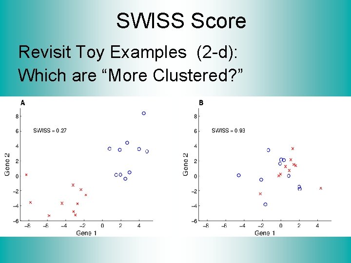
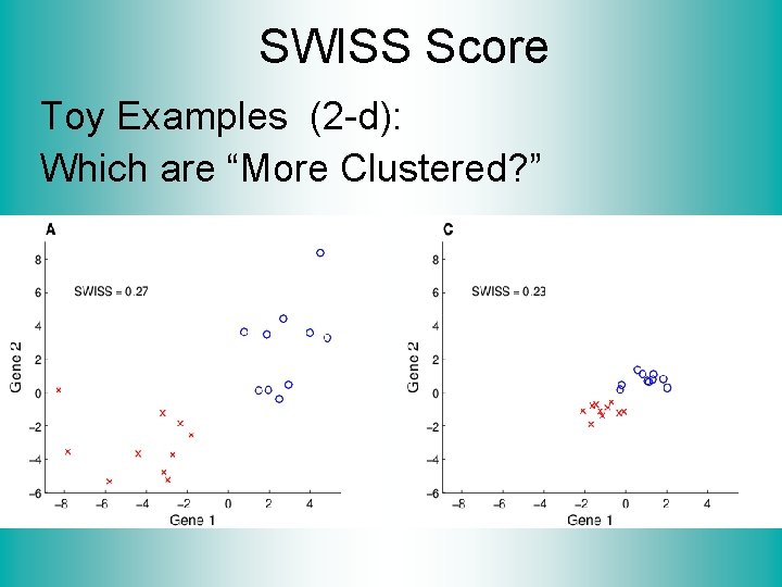
SWISS Score Another Application of CI (Cluster Index) Cabanski et al (2010) Idea: Use CI in bioinformatics to “measure quality of data preprocessing” Philosophy: Clusters Are Scientific Goal So Want to Accentuate Them

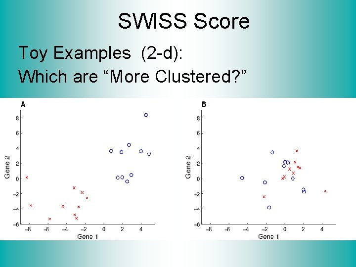
SWISS Score Toy Examples (2 -d): Which are “More Clustered? ”

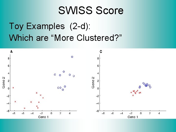
SWISS Score Toy Examples (2 -d): Which are “More Clustered? ”

SWISS Score •

SWISS Score •

SWISS Score •

SWISS Score •

SWISS Score •

SWISS Score Revisit Toy Examples (2 -d): Which are “More Clustered? ”

SWISS Score Toy Examples (2 -d): Which are “More Clustered? ”

SWISS Score Toy Examples (2 -d): Which are “More Clustered? ”

Participant Presentation Duyeol Lee PCA in Credit Risk Modelling