Chapter Five Factor Endowments and the HeckscherOhlin Theory

Chapter Five Factor Endowments and the Heckscher–Ohlin Theory 5. 1 Introduction In this chapter we extend our trade model in two important directions. First, we explain the basis for comparative advantage, that is, what determines comparative advantage. Second, we analyze the effect that international trade has on the earnings of factors of production in the two trading nations.

5. 2 Assumptions of the Theory As with other economic theories, the H–O theory presumes a number of simplifying conditions. We present together the presumptions that underlies theory and offer brief explanations to some of them. • the assumptions and their meanings 1. 2 N× 2 C× 2 F 2. Same technology in production 3. X and Y are labor intensive and capital intensive respectively 4. Under constant returns to scale in both nations 5. Incomplete specialization 6. Equal tastes in both nations 7. Perfect competition in both commodity and factor markets 8. Perfect factor mobility 9. No idle resources About the meanings of the assumptions, see page 117 -118.

5. 3 Factor Intensity, Factor Abundance, and the Shape of the Production Frontier Since H–O theory is expressed in terms of factor intensity and factor abundance, we deem it crucial to make these meanings clear and precise. 5. 3 A Factor Intensity • Factor intensity is described as the proportion of two factors of production in which they are used in producing different commodities. • For nation 1, K/L (means the ratio of capital to labor ) are ¼ and 1 for commodity X, Y respectively. Commodity X is L–intensive , Commodity Y is K–intensive. For nation 2 ……

• Note that even though commodity Y is K–intensive in relation to commodity X in both nations, Nation 2 uses a relatively higher K/L in the production of both X and Y. • The obvious question is: Why does nation 2 use more K– intensive production techniques in both commodities than in nation 1? The answer is capital must be relatively cheaper in nation 2 than in nation 1, so that producers in nation 2 will respond to use relatively more capital in producing both commodities to minimize their costs of production by substituting the cheaper factor of production（K）for the more expensive one (L).

• Another question: Why is capital relatively cheaper in nation 2? To answer this question, we must define factor abundance and examine its relationship to factor prices. • Before we explain factor abundance , I’d like to, at the end of this section, draw your attention to a point of crucial importance which, however, is not explicitly stated in average domestic textbooks: Strictly speaking , only if K/L in the production of Y exceeds that in the production of X at all possible relative factor prices can we say unequivocally that commodity Y is the K–intensive commodity.

5. 3 B Factor Abundance There are two ways to define factor abundance: • One way is in terms of physical units (i. e. , in terms of the overall amount of capital and labor available to each nation), defined as: Nation 2 is capital abundant if the ratio of the total amount of capital to the total amount of labor is greater than that in nation 1(i. e. , TK/TL for N 2 exceeds TK/TL for N 1). Note that it is not the absolute amount of capital and labor available in each nation that is important, but what really matters is the relative amount (the ratio of the total amount of capital to the total amount of labor)—a notion in relative sense. According to this definition, a nation can still be K abundant even if it has less capital.

• Another way is in terms of relative factor prices (i. e. , in terms of rental price of capital, r and the price of labor time, w in each nation. ), defined as: Nation 2 is capital abundant if the ratio of the rental price of capital to the price of labor time is lower than that in nation 1 (i. e. , PK/PL is smaller in nation 2 than in nation 1). Note once again that it is not the absolute level of r that determines whether or not a nation is K abundant, but the relative level r/w. • The relationship between the two definitions is clear: the former considers only the supply of factors while the latter both the supply and demand. Since we assume equal tastes or demand preference in both nations, the two definitions give the same conclusions from different angles. • Direct Vs. derived demand

• But this case is not always true in real world. There does exist a strong or week demand biased in favor of this or another commodity, which distorts the relative price levels. • If the spending pattern or consumption pattern in N 2 is strongly biased in favor of commodity Y which is capitalintensive, the derived demand for capital could be higher in N 2 and the price of capital r 2 could be higher enough. As a result, nation 2 is otherwise labor- abundant. This is how a biased spending pattern will distort the relative factor prices. In such situations it is the definition in terms of relative factor prices that should be used. That is, a nation is K abundant if the relative price of capital is lower in it than in the other nation.

5. 3 C Factor Abundance and the Shape of the Production Frontier We plot the production frontiers of nation 1 and nation 2 on the same set of axes in fig. 5. 2. . There is a biased expansion of production frontier, i. e. , the production frontier shifts out much more in one direction than in the other. • Since nation 1 is L abundant nation and commodity X is L–intensive, its production frontiers is skewed toward the horizontal axis, which measures commodity X, indicating that nation 1 can produce relatively more of X than nation 2. • Since nation 2 is K abundant nation and commodity Y is K–intensive, its production frontiers is biased toward the vertical axis, which measures commodity Y production, indicating that nation 2 can produce relatively more of Y than nation 1.

5. 4 Factor Endowment and the Heckscher– Ohlin Theory • Having clarified the meaning of factor intensity and factor abundance, we are now ready to present the modern theory of international trade: the H–O theory. This theory is also referred to as factor-proportions theory, because it emphasizes the interplay between the proportions in which different factors of production are available in different nations (factor abundance) and the proportions in which they are used in producing different goods (factor intensity).

• In a nutshell, the Heckscher–Ohlin theory can be presented in the forms of two theorems: 1. The so–called H–O theorem which deals with and predicts the pattern of trade. 2. The factor–price equalization theorem which deals with the effect of international trade on factor prices

5. 4 A The Heckscher–Ohlin Theorem • We state the Heckscher–Ohlin theorem as follows: A nation will export the commodity whose production requires the intensive use of the nation’s relatively abundant and cheap factor and import the commodity whose production requires the intensive use of the nation’s relatively scarce and expensive factor. In short, the relatively labor–rich nation exports the relatively labor– intensive commodity and imports the relatively capital–intensive commodity.

• Of all the possible reasons (technologic gap, differences in tastes, economy to scale and imperfect competition etc. ) for differences in relative commodity prices and comparative advantage among nations, the H–O theorem singles out the differences in factor abundance or factor endowments, among nations as the basic cause or determinant of comparative advantage and international trade. Thus, the H–O theorem goes one step forward to explain the comparative advantage rather than assuming the existence of it , as was the case for classical economists.

5. 4 B General Equilibrium Framework of the H–O Theorem We say the H–O model is a general equilibrium model for the reason that it takes all economic forces into considerations, these forces are at work together to determine the prices of final commodities. See fig. 5. 3. on page 126.

5. 4 C Illustration of the Heckscher–Ohlin Theory • Since we assume the two nations have equal tastes or demand preferences, they face the same indifference map. For simplicity, we assume the two nations are on the same indifference curve Ⅰ in isolation and end up on the same indifference curve Ⅱ of the indifference map. We only did so in order to facilitate the graphic illustration of fig. 5. 4. (this leaves the conclusion unaffected). Though, it need not be the case. • In fig. 5. 4. , the production frontiers of nation 1 and nation 2 are the very same ones as we have discussed in previous sections. • At any other relative price other than PB, trade is in imbalance and pressure from demand supply will give rise to the fall or rise of relative price, causing it to gravitate toward the equilibrium PB. • Explain the pattern of trade and gains from trade. Since the indifference curve Ⅱ is higher than curve Ⅰ, both nations’ welfares are improved.

5. 5 Factor–Price Equalization and Income Distribution • In the section 3. 5 B Equilibrium–Relative Commodity Prices with Trade, we learned that free trade tends to equalize commodity prices among trading partners. Can the same be said for factor prices? The answer is invariably “can”. • To answer it, we carry on to this section and examine the other form of theorem of the H–O theory, the factor–price equalization theorem, which is really a corollary of H–O theorem.

5. 5 A The Factor–Price Equalization Theorem • We state it as follows: International trade will bring about equalization in the relative and absolute returns to homogeneous factors across nations. As such, international trade is a substitute for the international mobility of factors. • What this means is that international trade will cause the wage rates of homogeneous labor and the interest rates of homogeneous capital to be the same in all trading nations (i. e. , w 1=w 2…, r 1=r 2). It also implies that both relative and absolute factor prices will be equalized(r 1/ w 1= r 2 / w 2). • Homogeneous labor and homogeneous capital

• Have a look into the process of the following example to see how wages are equalized by trade in two nations. In the absence of trade, the relative price of X is lower in nation 1 than in nation 2 because the relative price of labor or wage rate (w) is lower in nation 1 than in nation 2. Nation 1 Nation 2 W 1 is low W 1< W 2 is high 1. As it specializes in producing X and reduces Y: producing Y and reduces X: …………………………………… 2. relative D for labor rises, DL ↗ relative D for labor falls, DL ↘ …………………………………… 3. As a result, the rise in D for As a result, the fall in D for abundant factor L causes its scarce factor L causes its price to increase, that is, price to decrease, that is wage (w) to rise W 1 ↗ wage (w) to fall, W 2 ↘ …… 4. cheap factor L becomes expensive factor L becomes more expensive W 1= W 2 cheaper

This process continues until the W in nation 1 and nation 2 become equal. This proves that international trade tends to reduce the pre–trade differences in W between the two nations.

In like manner, we can prove that international trade tends to equalize the interest rate r in the two nations, too. Remember: This is left for you to do as an extra-class assignment.

5. 5 B Relative and Absolute Factor–Price Equalization • In the preceding Section 5. 5 A, we have proved that international trade tends to reduce the international differences in the returns to homogeneous factor. In this section we go further to demonstrate graphically that international trade would in fact bring about complete equalizations in relative factor prices when all the assumptions made in section 5. 2 A hold. • See fig. 5. 5. on page 132: Horizontal axis measures the relative price of labor (w/r), and vertical axis measures the relative price of commodity X(PX/PY). Since each nation operates under perfect competition and uses the same technology , there is a one-to-one corresponding relationship between w/r and PX/PY.

• Since in the absence of trade, w/r is lower in nation 1 than in nation 2, nation 1 has a comparative advantage in X and nation 2 has a comparative advantage in Y. Nation 1 Nation 2 (w/r)1 is low (w/r)1 < (w/r)2 is high 1. As it specializes in producing X and reduces Y: producing Y and reduces X: 2. DL increases relative to DK , DL decreases in relation to DK 3. cause (w/r)1 to rise, (w/r)1 ↗ cause (w/r)2 to fall, (w/r)2 ↘ …… (w/r)1= (w/r)2 • This process continues until PB=PB' ，(w/r)1= (w/r)2 in both nations. • To summarize, PX/PY will become equal as a result of international trade, and this will occur only when w/r has also become equal in the two nations.

So far we have showed the process by which relative factor prices are equalized. • We now move on to take a look at how absolute factor prices becomes equalized by trade. Equalization of absolute factor prices means free international trade also equalizes the real wages for the same type of labor in the two nations and the real rate of interest for the same type of capital in the two nations (as is discussed in the Section 5. 5 A). This, however, presumes that all the assumptions hold: perfect competition in both commodity and factor markets, same technology, constant returns to scale in the production of both commodities.

• From section 5. 5 A and 5. 5 B we can say that trade acts as a substitute for the international mobility of factors of production in the sense that they have the same effects on factor prices. That is, trade serves as an indirect way of trading factors of production. • Factors of production, be it labor or capital, is in constant pursuit of their own interests. Given perfect mobility, labor would shift or migrate from the lowwage nation to high-wage nation until the returns to the same type of labor became equal. Similarly, capital would move from low-interest rate nation to high-interest nation until returns on….

5. 5 C Effect of Trade on the Distribution of Income • While in previous section we examined the effect of international trade on the difference in factor prices between nations, in this section we analyze the effect of international trade on relative factor prices and income distribution within each nation. That is, we examine how international trade affects the real wages and real income of labor in relation to real interest rates and the real income of owners of capital within each nation.

• Since resources—capital and labor, are assumed to be fully utilized, both before and after trade, the real income of labor moves in the same direction as the movement of the price of labor, and the real income of capital moves in the same direction as the movement of the price of capital. • From Section 5. 5 A on P 129, we can reach the conclusion that: International trade causes the real income of the nation’s abundant and cheap factor to rise, and causes the real income of the nation’s scarce and expensive factor to fall —referred to as Stolper-Samuelson theorem (斯托伯－萨 谬尔森定理).

A question for in-class discussion: Why do labor unions in developed nations generally lobby against the imports from the developing countries?

While nations generally gains from international trade, however, it is quite possible that international trade may hurt particular groups within nations—in other words, that international trade will have strong and uneven effects on the distribution of income. The benefits received by owners of capital tends to more than offset the losses that labor suffer due to trade. Labor union speak for the labor and lobby for trade restrictions. Should the U. S. government implement trade restrictions? The answer is no! for an individual interests group…, for the nation as a whole…With an appropriate redistribution policy on the part of the gov. , both labor and owners of capital can benefit from free international trade— to transfer part of the gains to subsidize the labor.

5. 5 D The Specific-Factor Model • In the previous section we have discussed the effect that inter-national trade has on the distribution of income. But this effect is based on assumption 8( that factors are perfectly mobile within a nation from one industry or sector to another). This is likely to be true in the long run. In the short run, however, it may not be true when some factors are immobile or specific to some industry or sector (a factor is industry-specific or sector-specific). In such a case we have to modify the conclusions of the H-O theory on the effect of international trade on the distribution of income. We introduce the specific-factor model to explain the effect.

• What is a specific factor? A factor is specific to some industry or commodity if they can be used only in the production of the particular commodity. • In practice, factor specificity is not a permanent condition. Rather, it is a matter of time or a question of the speed of adjustment and the distinction between specific and mobile factors is not a sharp line. The more specific a factor is, the longer it takes to re-deploy the factor between industries.

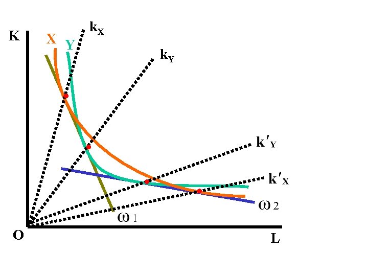
w. Y w. X E · w OX LX L w LY OY

w. Y w. X E · w OX LX L w LY OY

w. Y w. X · E′ · E · F w′ w OX LX L L′ w′ w LY OY

• Effect of trade on the short-run distribution of income within a nation—the specific-factor model • From basic microeconomics we know that under perfect competition and in isolation, the value of the marginal product of labor in the production of X (VMPLX, the returns to factor ) in the two industries in Nation 1 are : VMPLX = PX MPLX VMPKX = PX MPKX …………………………………………… VMPLY = PY MPLY VMPKY =PY MPKY • VMPLX is equal to the price of X (PX)times the marginal product of labor (MPLX). For producers to maximize profits, they will employ labor(capital) until the wage(interest rate) they must pay equals the value of the marginal product of labor(capital) wx =VMPLX w. Y =VMPLY ; r. X= VMPKX r. Y =VMPKY

• And such, we get the following expressions wx = PX MPLX r. X= PX MPKX w. Y = PY MPLY r. Y = PY MPKY • Suppose Nation 1 is labor-abundant nation , commodity X is Lintensive, labor is perfectly mobile between two industries, but capital is specific. With the opening of trade, Nation 1 will specializes in producing X and PX/PY will rise. We suppose again for simplicity that PX increases while PY remain unchanged. 1. Change in the nominal wage rate or nominal income of labor • As the increase in PX/PY will increases the demand for and the nominal wage rate of labor in industry X, wx ↗. Industry Y will have to pay a higher going nominal wage rate with the transfer of some of its labor to the production of X, w. Y ↗. • Since labor is perfectly mobile , the wage of labor will be the same in the production of commodities X and Y. wx = w. Y =w.

2. Change in the real wage rate or real income of labor • From principles of microeconomics we know the law of diminishing returns is at work as labor migrates from industry Y to X. If industry X employs more L with a given amount of K, MPLX declines(MPLX↘). It follows that although w and PX increase, the increase in w is less than the increase in PX. The real wage rate w/ PX declines in industry X. For industry Y, MPLY ↗, the real wage rate w/ PY rises. • The effect of this on the real wage rate of labor in nation 1 thus is ambiguous(depends on their spending pattern). It falls in terms of X but rises in terms of Y, which means that the real wage rate and income will fall for workers who consumes mainly X and will increase for workers who consumes mainly Y.

Let us take some time out to briefly review the law of diminishing returns before we can turn to the analysis. The law of diminishing returns holds that we will get less and less extra output when we add successively additional units of an input, while holding other inputs constant. Or to put it the other way around, the marginal product (MP) of each unit of input will decline as the amount of that input increases, all other inputs held fixed.

3. Change in the rewards(returns) to capital-the specific factor The returns to the specific factor(capital) change unambiguously. In the production of X, since the specific capital(K) has more labor to work with, MPKX ↗, i. e. , the real income of immobile K increases, rx/PX ↗in the industry X. In the production of Y, since the specific capital(K) has less labor to work with, MPKX ↘, i. e. , the real income of immobile K decreases, r. Y/PY ↘ in the industry Y.

• We generalize the specific-factors model as follows : trade will have an ambiguous effect on the nation’s mobile factors, benefit the immobile factors specific to the nation’s export commodities or sectors, and harm the immobile factors specific to the nation’s import-competing commodities or sectors. • The long-run VS. the short-run The conclusion above reached by the specific-factors model is what we can expect in the short-run when some factors are specific or immobile. In the long-run, however, all factors are perfectly mobile, and the conclusion is exactly as the H-O theory postulates (that is, the opening of trade will lead to an increase in the real income or return of the factors used intensively in the nation’s export commodities and to a reduction in the real income or return of the factors used intensively in the nation’s importcompeting commodities).

5. 6 Empirical Tests of the H-O Model 5. 6 A Empirical Results—The Leontief Paradox • The first empirical test of the H-O model was made by Leontief. The results were startling and seemed to conflict with the H-O theory. Ever since, a large number of empirical tests were conducted in an attempt to reconcile the results with the model. • For his test, Leontief utilized the input-output table of the U. S. economy to calculate the amount of L and K in a “representative bundle” of $1 million worth of exports and import substitutes for the year 1947 (the reason why Leontief used U. S. data on import substitutes was that foreign production data on actual U. S. imports were unavailable).

• The Leontief Paradox Since the U. S. was accepted as the most K-abundant nation in the world, Leontief expected to find that U. S. would export K-intensive commodities and import Lintensive commodities. But the results went the other way around— U. S. import substitutes were more Kintensive than U. S. exports, that is, the U. S. seemed to import K-intensive commodities and export L- intensive commodities. This was the opposite of what the H-O model predicted, and the result becomes known as the Leontief Paradox. • It is the single biggest piece of evidence against the H-O theory.

5. 6 B Explanations of the Leontief Paradox There are more than one sources of bias as follows 1. Natural resources — oversimplified model of two factors, K and L.

2. Tariff policy implemented by U. S. government —A tariff is nothing else than a tax levied when a good is imported. And such, a tariff reduces imports and stimulates the domestic production of import substitutes. The fact biased the pattern of trade that L-intensive industries were heavily protected, and reduced the L-intensity of U. S. import substitutes.

3. Physical capital—perhaps the most important source of bias. Human capital and knowledge capital were completely ignored in his measurement of capital. Human capital refers to education, job training, and health embodied in workers, which increase their productivity. The implication is that since U. S. labor embodies more human capital than foreign labor, if we incorporate human capital component to physical capital, U. S. exports would be more K-intensive in relation to its import substitutes

5. 6 C Factor-intensity reversal 1. Factor-intensity reversal —a situation where a given commodity is L-intensive in the L-abundant nation and K-intensive in the K-abundant nation.

2. The elasticity of substitution of factors in production measures the degree or ease with which one factor can be substituted for another in production as the relative price of the factor declines.

3. The result of factor-intensive reversal When factor-intensity reversal is present, neither the H-O theorem nor the factor-price equalization theorem holds. The H-O model fails because it would predict that Nation 1 (the L-abundant nation) would export commodity X (its L-intensive commodity) and that Nation 2 (the K-abundant nation) would also export commodity X (its K-intensive commodity). Since the two nations cannot possibly export the same homogeneous commodity to each other, the H-O model no longer predicts the pattern of trade.