Chapter 7 Numerical Differentiation and Integration INTRODUCTION DIFFERENTIATION

Chapter 7 Numerical Differentiation and Integration

INTRODUCTION DIFFERENTIATION USING DIFFERENCE OPREATORS DIFFERENTIATION USING INTERPOLATION RICHARDSON’S EXTRAPOLATION METHOD NUMERICAL INTEGRATION

NEWTON-COTES INTEGRATION FORMULAE THE TRAPEZOIDAL RULE ( COMPOSITE FORM ) SIMPSON’S RULES ( COMPOSITE FORM ) ROMBERG’S INTEGRATION DOUBLE INTEGRATION

Basic Issues in Integration What does an integral represent? = AREA = VOLUME

NUMERICAL INTEGRATION Consider the definite integral

Then, if n = 2, the integration takes the form

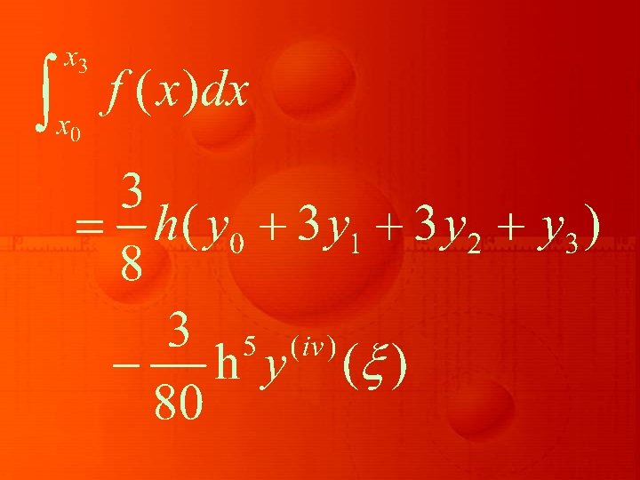
Thus Simpson’s 1/3 rule is based on fitting three points with a quadratic. Similarly, for n = 3, the integration is found to be

This is known as Simpson’s 3/8 rule, which is based on fitting four points by a cubic. Still higher order Newton. Cotes integration formulae can be derived for large values of n.

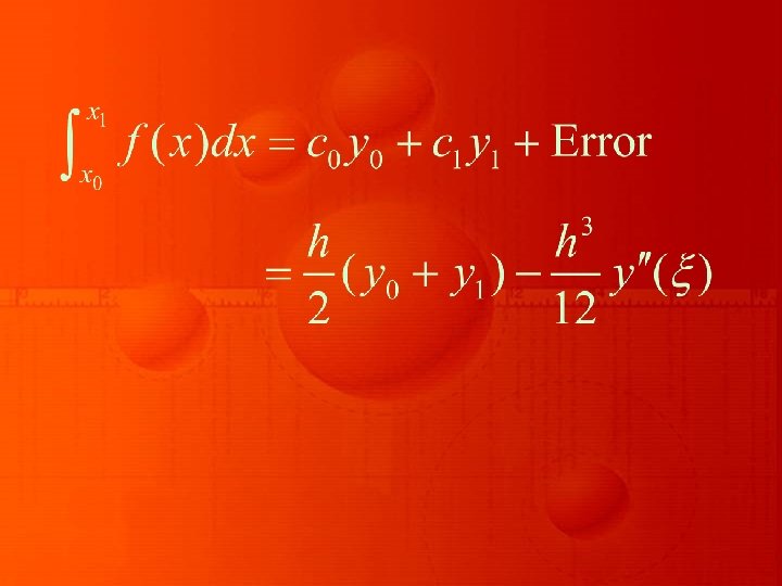
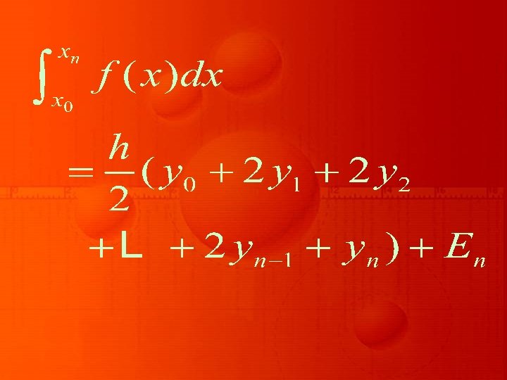
TRAPEZOIDAL RULE

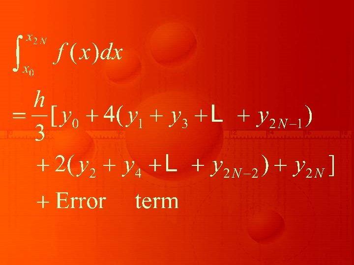
SIMPSON’S 1/3 RULE

Simpson’s 3/8 rule is

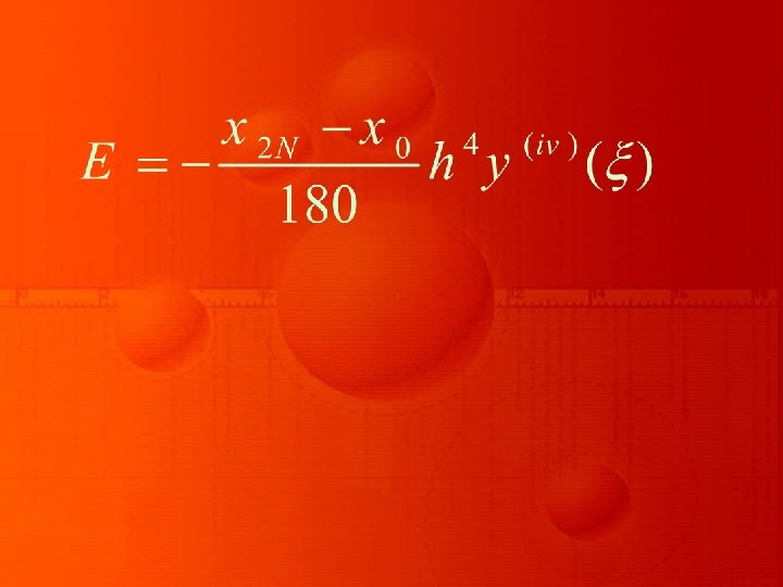
with the global error E given by

ROMBERG’S INTEGRATION We have observed that the trapezoidal rule of integration of a definite integral is of O(h 2), while that of Simpson’s 1/3 and 3/8 rules are of fourthorder accurate.

We can improve the accuracy of trapezoidal and Simpson’s rules using Richardson’s extrapolation procedure which is also called Romberg’s integration method.

For example, the error in trapezoidal rule of a definite integral

can be written in the form

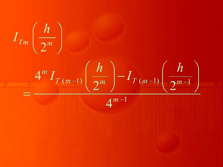
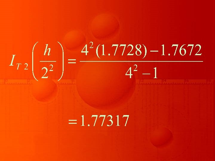
By applying Richardson’s extrapolation procedure to trapezoidal rule, we obtain the following general formula

where m = 1, 2, … , with IT 0 (h) = IT (h). For illustration, we consider the following example.

Example: Using Romberg’s integration method, find the value of starting with trapezoidal rule, for the tabular values

x 1. 0 1. 1 1. 2 1. 3 1. 4 1. 5 1. 6 1. 7 1. 8 y = f(x) 1. 543 1. 669 1. 811 1. 971 2. 151 2. 352 2. 577 2. 828 3. 107

Solution Taking

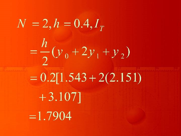
Let IT denote the integration by Trapezoidal rule, then for

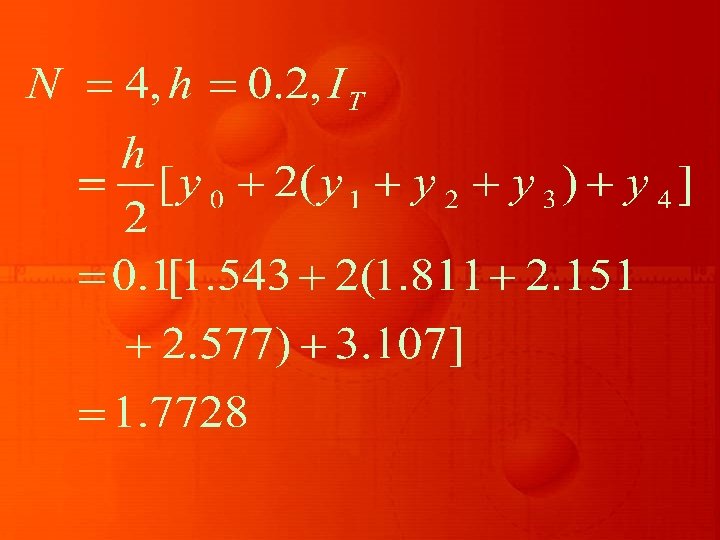
Similarly for

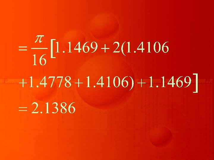
Now, using Romberg’s formula , we have

Thus, after three steps, it is found that the value of the tabulated integral is 1. 7671.

DOUBLE INTEGRATION To evaluate numerically a double integral of the form

over a rectangular region bounded by the lines x = a, x = b, y = c, y = d we shall employ either trapezoidal rule or Simpson’s rule, repeatedly With respect to one variable at a time.

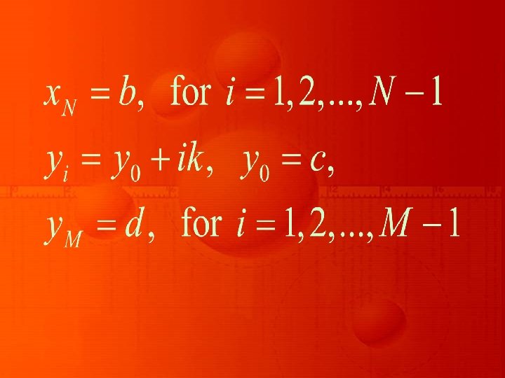
Noting that, both the integrations are just a linear combination of values of the given function at different values of the independent variable, we divide the interval [a, b] into N equal

sub-intervals of size h, such that h = (b – a)/N; and the interval (c, d) into M equal sub-intervals of size k, so that k = (d – c)/M. Thus, we have

Thus, we can generate a table of values of the integrand, and the above procedure of integration is illustrated by considering a couple of examples.

Example Evaluate the double integral by using trapezoidal rule, with h = k = 0. 25.

Solution Taking x = 1, 1. 25, 1. 50, 1. 75, 2. 0 and y = 1, 1. 25, 1. 50, 1. 75, 2. 0, the following table is generated using the integrand

x y 1. 00 1. 25 1. 50 1. 75 2. 00 1. 00 0. 5 0. 4444 0. 3636 0. 3333 1. 25 0. 4444 0. 3636 0. 3333 0. 3077 1. 50 0. 4 0. 3636 0. 3333 0. 3077 0. 2857 1. 75 0. 3636 0. 3333 0. 307 0. 2667 2. 00 0. 3333 0. 3077 0. 2857 0. 2667 0. 2857 0. 25

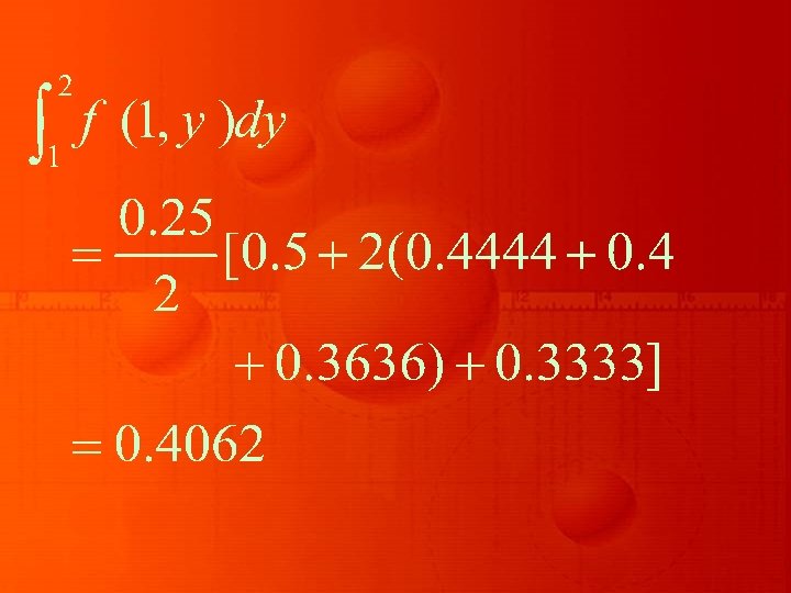
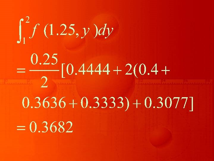
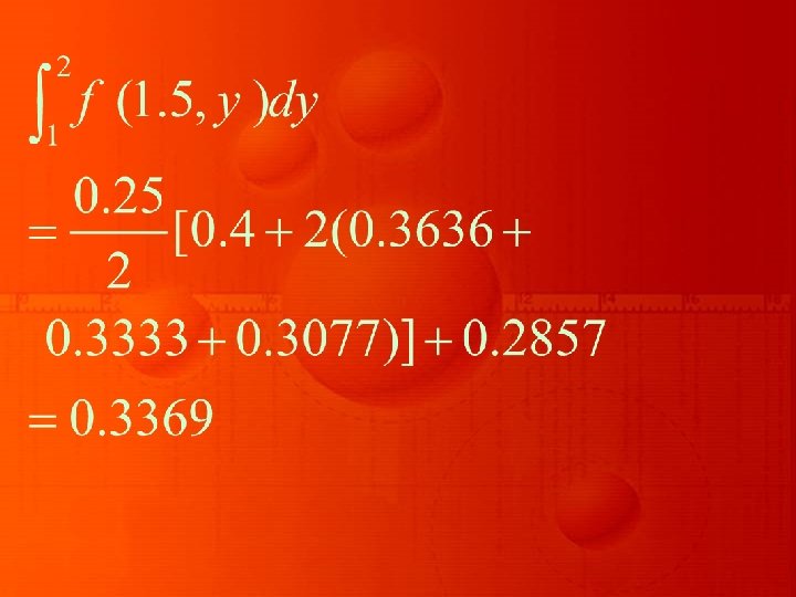
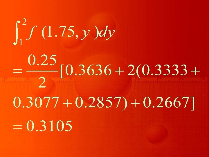
Keeping one variable say x fixed and varying the variable y, the application of trapezoidal rule to each row in the above table gives

and

Therefore,

By use of the last equations we get the required result as

Example : Evaluate by numerical double integration.

Solution Taking x = y = π/4, 3 π /8, π /2, we can generate the following table of the integrand

x y 0 π/8 π/4 0 0. 0 π/8 0. 6186 0. 8409 0. 9612 π/4 0. 8409 0. 9612 3π/8 0. 9612 1. 0 π/2 1. 0 3π/8 0. 6186 0. 8409 0. 9612 1. 0 π/2 1. 0 0. 9612 0. 8409 0. 6186 0. 0

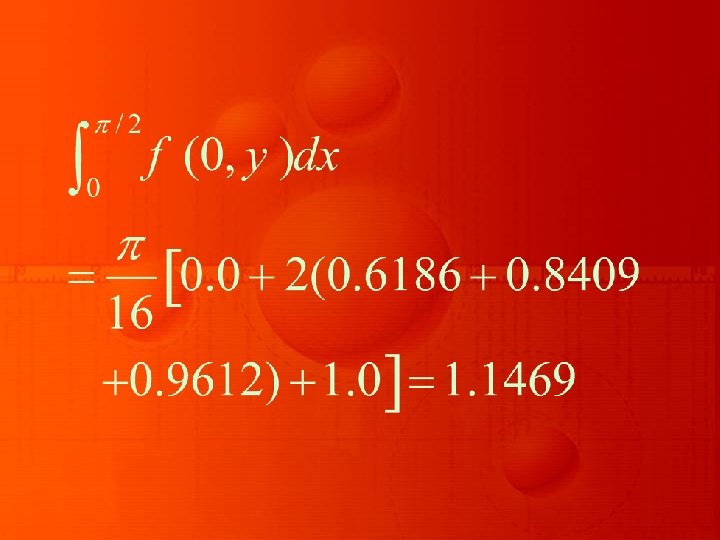
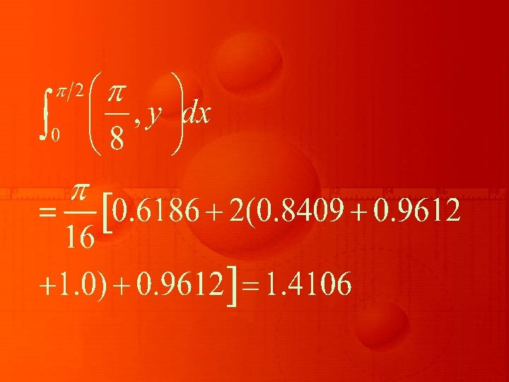
Keeping one variable as say x fixed and y as variable, and applying trapezoidal rule to each row of the above table, we get

Similarly, we get

and

Using these results, we finally obtain