Chapter 1 Functions GoldsteinSchneiderLayAsmar CALCULUS AND ITS APPLICATIONS

Chapter 1 Functions Goldstein/Schneider/Lay/Asmar, CALCULUS AND ITS APPLICATIONS, 11 e – Slide 1 of 115

Chapter Outline q The Slope of a Straight Line q The Slope of a Curve at a Point q The Derivative q Limits and the Derivative q Differentiability and Continuity q Some Rules for Differentiation q More About Derivatives q The Derivative as a Rate of Change Goldstein/Schneider/Lay/Asmar, CALCULUS AND ITS APPLICATIONS, 11 e – Slide 2 of 115

§ 1. 1 The Slope of a Straight Line Goldstein/Schneider/Lay/Asmar, CALCULUS AND ITS APPLICATIONS, 11 e – Slide 3 of 115

Section Outline q Nonvertical Lines q Positive and Negative Slopes of Lines q Interpretation of a Graph q Properties of the Slope of a Nonvertical Line q Finding the Slope and y-Intercept of a Line q Sketching the Graph of a Line q Making Equations of Lines q Slope as a Rate of Change Goldstein/Schneider/Lay/Asmar, CALCULUS AND ITS APPLICATIONS, 11 e – Slide 4 of 115

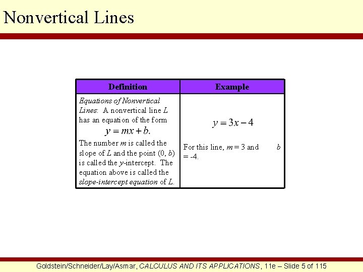
Nonvertical Lines Definition Example Equations of Nonvertical Lines: A nonvertical line L has an equation of the form The number m is called the slope of L and the point (0, b) is called the y-intercept. The equation above is called the slope-intercept equation of L. For this line, m = 3 and = -4. b Goldstein/Schneider/Lay/Asmar, CALCULUS AND ITS APPLICATIONS, 11 e – Slide 5 of 115

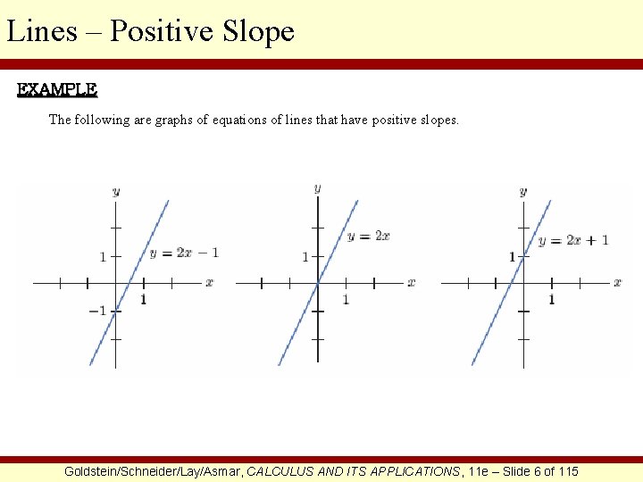
Lines – Positive Slope EXAMPLE The following are graphs of equations of lines that have positive slopes. Goldstein/Schneider/Lay/Asmar, CALCULUS AND ITS APPLICATIONS, 11 e – Slide 6 of 115

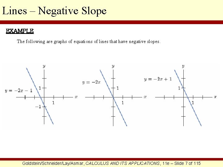
Lines – Negative Slope EXAMPLE The following are graphs of equations of lines that have negative slopes. Goldstein/Schneider/Lay/Asmar, CALCULUS AND ITS APPLICATIONS, 11 e – Slide 7 of 115

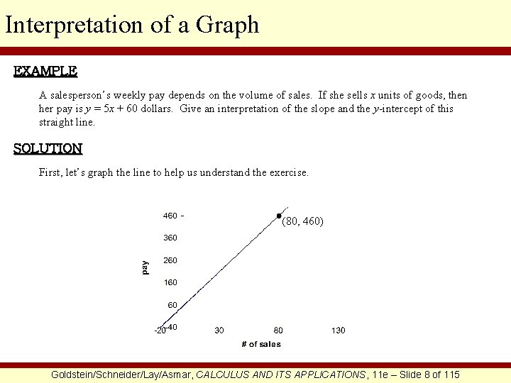
Interpretation of a Graph EXAMPLE A salesperson’s weekly pay depends on the volume of sales. If she sells x units of goods, then her pay is y = 5 x + 60 dollars. Give an interpretation of the slope and the y-intercept of this straight line. SOLUTION First, let’s graph the line to help us understand the exercise. (80, 460) Goldstein/Schneider/Lay/Asmar, CALCULUS AND ITS APPLICATIONS, 11 e – Slide 8 of 115

Interpretation of a Graph CONTINUED The slope is 5, or 5/1. Since the numerator of this fraction represents the amount of change in her pay relative to the amount of change in her sales, the denominator, for every 1 sale that she makes, her pay increases by 5 dollars. The y-intercept is 60 and occurs on the graph at the point (0, 60). This point suggests that when she has executed 0 sales, her pay is 60 dollars. This $60 could be referred to as her base pay. Goldstein/Schneider/Lay/Asmar, CALCULUS AND ITS APPLICATIONS, 11 e – Slide 9 of 115

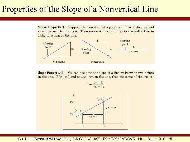
Properties of the Slope of a Nonvertical Line Goldstein/Schneider/Lay/Asmar, CALCULUS AND ITS APPLICATIONS, 11 e – Slide 10 of 115

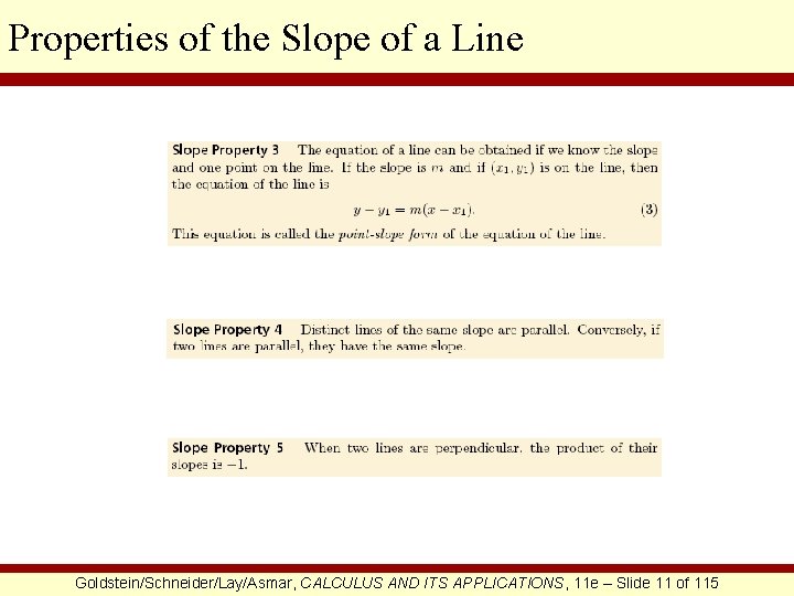
Properties of the Slope of a Line Goldstein/Schneider/Lay/Asmar, CALCULUS AND ITS APPLICATIONS, 11 e – Slide 11 of 115

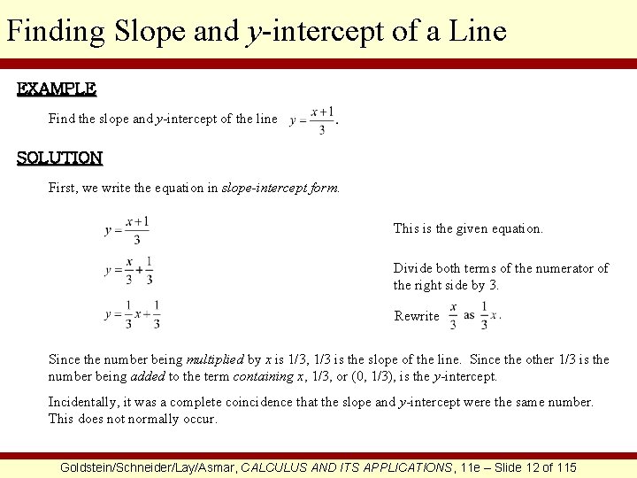
Finding Slope and y-intercept of a Line EXAMPLE Find the slope and y-intercept of the line SOLUTION First, we write the equation in slope-intercept form. This is the given equation. Divide both terms of the numerator of the right side by 3. Rewrite Since the number being multiplied by x is 1/3, 1/3 is the slope of the line. Since the other 1/3 is the number being added to the term containing x, 1/3, or (0, 1/3), is the y-intercept. Incidentally, it was a complete coincidence that the slope and y-intercept were the same number. This does not normally occur. Goldstein/Schneider/Lay/Asmar, CALCULUS AND ITS APPLICATIONS, 11 e – Slide 12 of 115

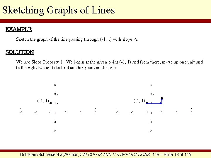
Sketching Graphs of Lines EXAMPLE Sketch the graph of the line passing through (-1, 1) with slope ½. SOLUTION We use Slope Property 1. We begin at the given point (-1, 1) and from there, move up one unit and to the right two units to find another point on the line. (-1, 1) Goldstein/Schneider/Lay/Asmar, CALCULUS AND ITS APPLICATIONS, 11 e – Slide 13 of 115

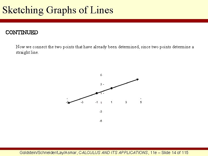
Sketching Graphs of Lines CONTINUED Now we connect the two points that have already been determined, since two points determine a straight line. Goldstein/Schneider/Lay/Asmar, CALCULUS AND ITS APPLICATIONS, 11 e – Slide 14 of 115

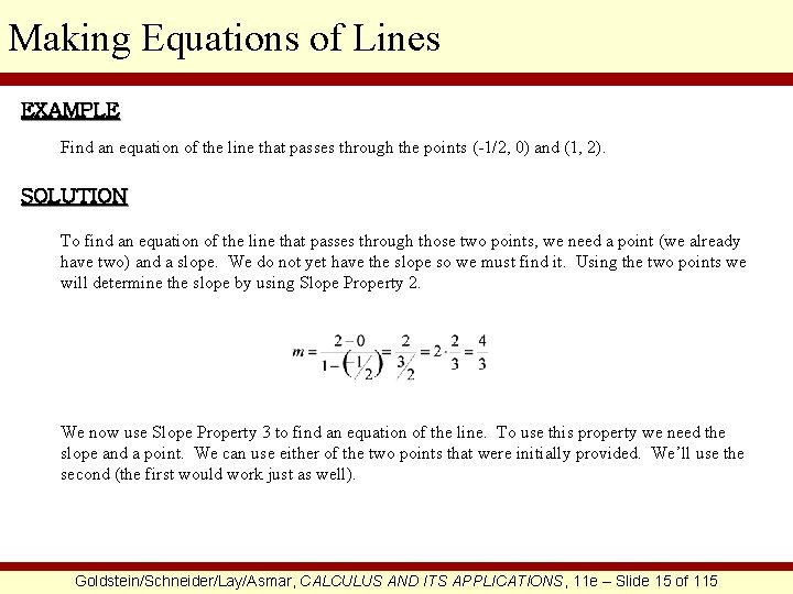
Making Equations of Lines EXAMPLE Find an equation of the line that passes through the points (-1/2, 0) and (1, 2). SOLUTION To find an equation of the line that passes through those two points, we need a point (we already have two) and a slope. We do not yet have the slope so we must find it. Using the two points we will determine the slope by using Slope Property 2. We now use Slope Property 3 to find an equation of the line. To use this property we need the slope and a point. We can use either of the two points that were initially provided. We’ll use the second (the first would work just as well). Goldstein/Schneider/Lay/Asmar, CALCULUS AND ITS APPLICATIONS, 11 e – Slide 15 of 115

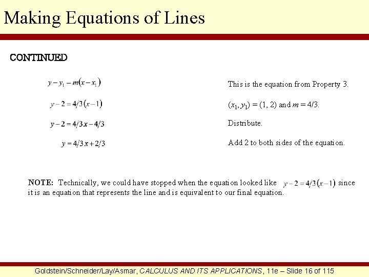
Making Equations of Lines CONTINUED This is the equation from Property 3. (x 1, y 1) = (1, 2) and m = 4/3. Distribute. Add 2 to both sides of the equation. NOTE: Technically, we could have stopped when the equation looked like it is an equation that represents the line and is equivalent to our final equation. Goldstein/Schneider/Lay/Asmar, CALCULUS AND ITS APPLICATIONS, 11 e – Slide 16 of 115 since

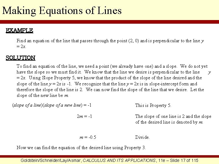
Making Equations of Lines EXAMPLE Find an equation of the line that passes through the point (2, 0) and is perpendicular to the line y = 2 x. SOLUTION To find an equation of the line, we need a point (we already have one) and a slope. We do not yet have the slope so we must find it. We know that the line we desire is perpendicular to the line y = 2 x. Using Slope Property 5, we know that the product of the slope of the line desired and the slope of the line y = 2 x is -1. We recognize that the line y = 2 x is in slope-intercept form and therefore the slope of the line is 2. We can now find the slope of the line that we desire. Let the slope of the new line be m. (slope of a line)(slope of a new line) = -1 2 m = -1 m = -0. 5 This is Property 5. The slope of one line is 2 and the slope of the desired line is denoted by m. Divide. Now we can find the equation of the desired line using Property 3. Goldstein/Schneider/Lay/Asmar, CALCULUS AND ITS APPLICATIONS, 11 e – Slide 17 of 115

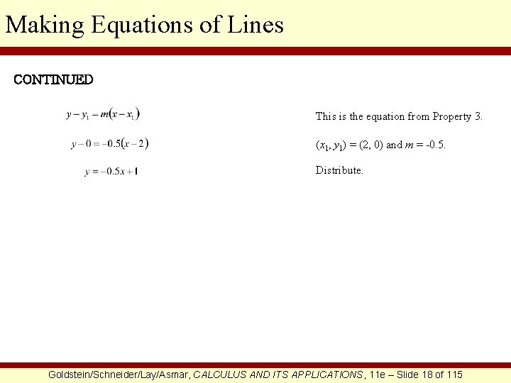
Making Equations of Lines CONTINUED This is the equation from Property 3. (x 1, y 1) = (2, 0) and m = -0. 5. Distribute. Goldstein/Schneider/Lay/Asmar, CALCULUS AND ITS APPLICATIONS, 11 e – Slide 18 of 115

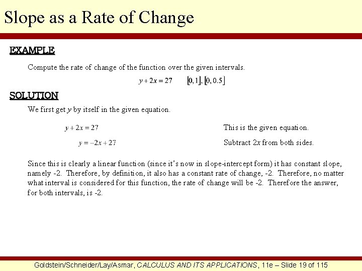
Slope as a Rate of Change EXAMPLE Compute the rate of change of the function over the given intervals. SOLUTION We first get y by itself in the given equation. This is the given equation. Subtract 2 x from both sides. Since this is clearly a linear function (since it’s now in slope-intercept form) it has constant slope, namely -2. Therefore, by definition, it also has a constant rate of change, -2. Therefore, no matter what interval is considered for this function, the rate of change will be -2. Therefore the answer, for both intervals, is -2. Goldstein/Schneider/Lay/Asmar, CALCULUS AND ITS APPLICATIONS, 11 e – Slide 19 of 115

§ 1. 2 The Slope of a Curve at a Point Goldstein/Schneider/Lay/Asmar, CALCULUS AND ITS APPLICATIONS, 11 e – Slide 20 of 115

Section Outline q Tangent Lines q Slopes of Curves q Slope of a Curve as a Rate of Change q Interpreting the Slope of a Graph q Finding the Equation and Slope of the Tangent Line of a Curve Goldstein/Schneider/Lay/Asmar, CALCULUS AND ITS APPLICATIONS, 11 e – Slide 21 of 115

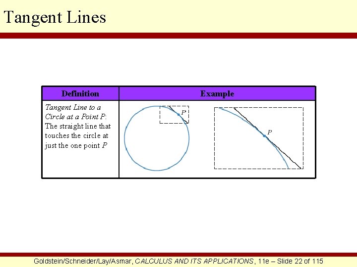
Tangent Lines Definition Example Tangent Line to a Circle at a Point P: The straight line that touches the circle at just the one point P Goldstein/Schneider/Lay/Asmar, CALCULUS AND ITS APPLICATIONS, 11 e – Slide 22 of 115

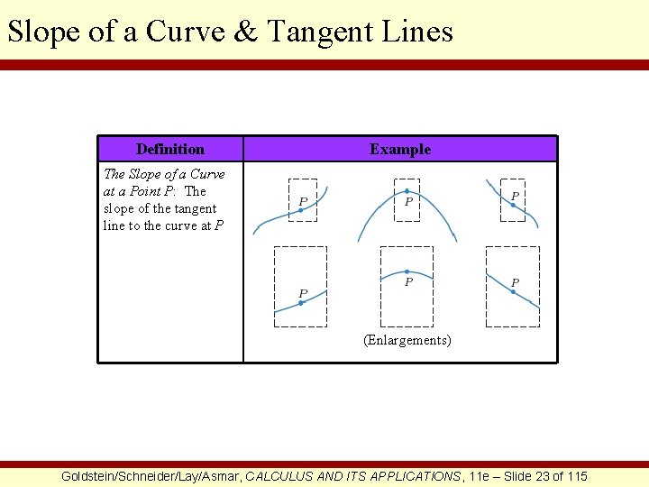
Slope of a Curve & Tangent Lines Definition Example The Slope of a Curve at a Point P: The slope of the tangent line to the curve at P (Enlargements) Goldstein/Schneider/Lay/Asmar, CALCULUS AND ITS APPLICATIONS, 11 e – Slide 23 of 115

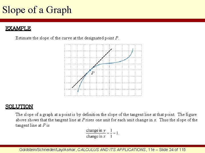
Slope of a Graph EXAMPLE Estimate the slope of the curve at the designated point P. SOLUTION The slope of a graph at a point is by definition the slope of the tangent line at that point. The figure above shows that the tangent line at P rises one unit for each unit change in x. Thus the slope of the tangent line at P is Goldstein/Schneider/Lay/Asmar, CALCULUS AND ITS APPLICATIONS, 11 e – Slide 24 of 115

Slope of a Curve: Rate of Change Goldstein/Schneider/Lay/Asmar, CALCULUS AND ITS APPLICATIONS, 11 e – Slide 25 of 115

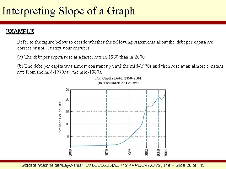
Interpreting Slope of a Graph EXAMPLE Refer to the figure below to decide whether the following statements about the debt per capita are correct or not. Justify your answers. (a) The debt per capita rose at a faster rate in 1980 than in 2000. (b) The debt per capita was almost constant up until the mid-1970 s and then rose at an almost constant rate from the mid-1970 s to the mid-1980 s. Goldstein/Schneider/Lay/Asmar, CALCULUS AND ITS APPLICATIONS, 11 e – Slide 26 of 115

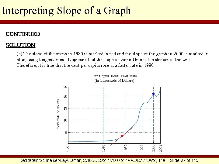
Interpreting Slope of a Graph CONTINUED SOLUTION (a) The slope of the graph in 1980 is marked in red and the slope of the graph in 2000 is marked in blue, using tangent lines. It appears that the slope of the red line is the steeper of the two. Therefore, it is true that the debt per capita rose at a faster rate in 1980. Goldstein/Schneider/Lay/Asmar, CALCULUS AND ITS APPLICATIONS, 11 e – Slide 27 of 115

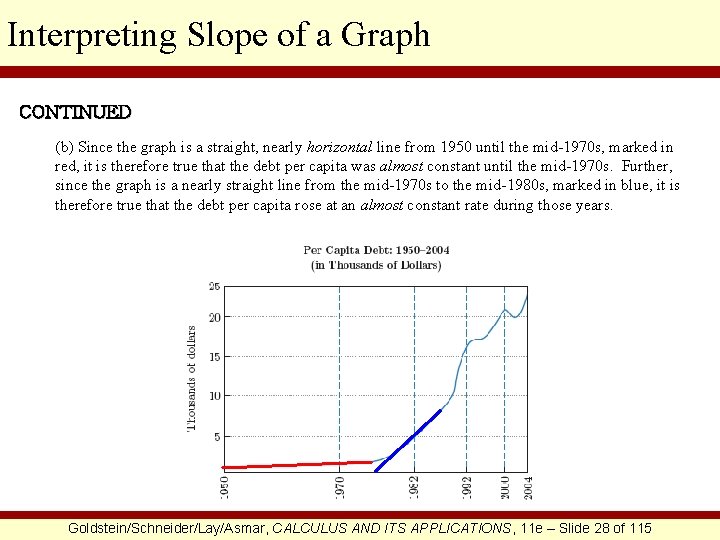
Interpreting Slope of a Graph CONTINUED (b) Since the graph is a straight, nearly horizontal line from 1950 until the mid-1970 s, marked in red, it is therefore true that the debt per capita was almost constant until the mid-1970 s. Further, since the graph is a nearly straight line from the mid-1970 s to the mid-1980 s, marked in blue, it is therefore true that the debt per capita rose at an almost constant rate during those years. Goldstein/Schneider/Lay/Asmar, CALCULUS AND ITS APPLICATIONS, 11 e – Slide 28 of 115

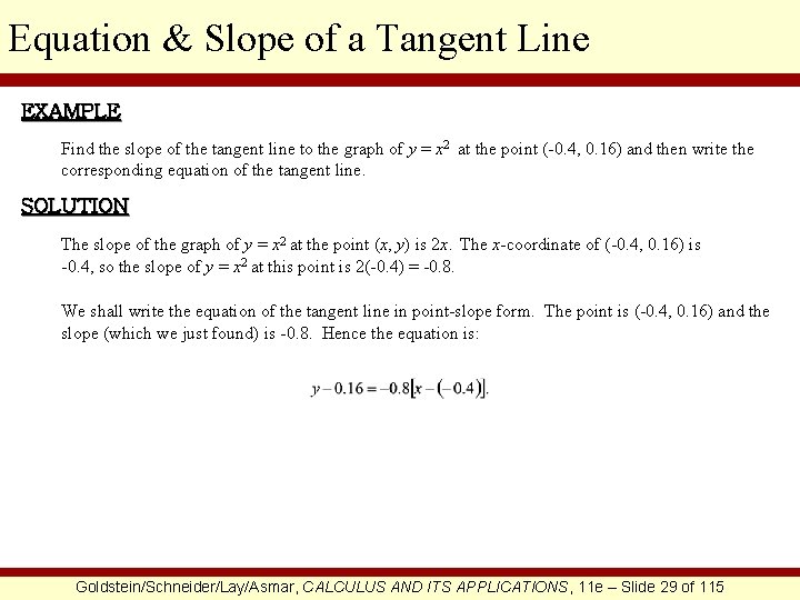
Equation & Slope of a Tangent Line EXAMPLE Find the slope of the tangent line to the graph of y = x 2 at the point (-0. 4, 0. 16) and then write the corresponding equation of the tangent line. SOLUTION The slope of the graph of y = x 2 at the point (x, y) is 2 x. The x-coordinate of (-0. 4, 0. 16) is -0. 4, so the slope of y = x 2 at this point is 2(-0. 4) = -0. 8. We shall write the equation of the tangent line in point-slope form. The point is (-0. 4, 0. 16) and the slope (which we just found) is -0. 8. Hence the equation is: Goldstein/Schneider/Lay/Asmar, CALCULUS AND ITS APPLICATIONS, 11 e – Slide 29 of 115

§ 1. 3 The Derivative Goldstein/Schneider/Lay/Asmar, CALCULUS AND ITS APPLICATIONS, 11 e – Slide 30 of 115

Section Outline q The Derivative q Differentiation q Slope and the Derivative q Equation of the Tangent Line to the Graph of y = f (x) at (a, f (a)) q Leibniz Notation for Derivatives q Calculating Derivatives Via the Difference Quotient q Differentiable q Limit Definition of the Derivative q Limit Calculation of the Derivative Goldstein/Schneider/Lay/Asmar, CALCULUS AND ITS APPLICATIONS, 11 e – Slide 31 of 115

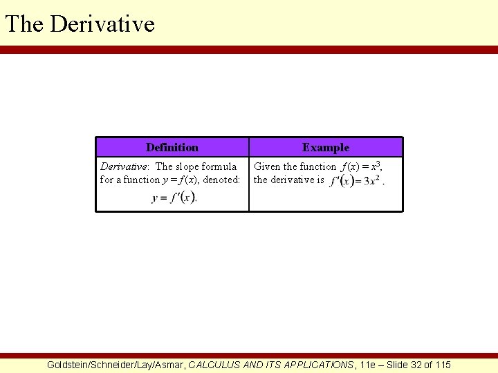
The Derivative Definition Derivative: The slope formula for a function y = f (x), denoted: Example Given the function f (x) = x 3, the derivative is Goldstein/Schneider/Lay/Asmar, CALCULUS AND ITS APPLICATIONS, 11 e – Slide 32 of 115

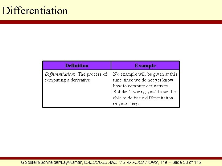
Differentiation Definition Example Differentiation: The process of computing a derivative. No example will be given at this time since we do not yet know how to compute derivatives. But don’t worry, you’ll soon be able to do basic differentiation in your sleep. Goldstein/Schneider/Lay/Asmar, CALCULUS AND ITS APPLICATIONS, 11 e – Slide 33 of 115

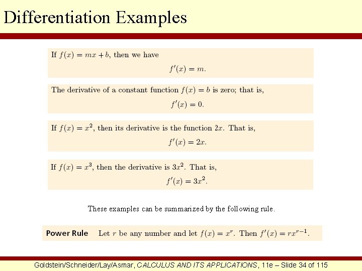
Differentiation Examples These examples can be summarized by the following rule. Goldstein/Schneider/Lay/Asmar, CALCULUS AND ITS APPLICATIONS, 11 e – Slide 34 of 115

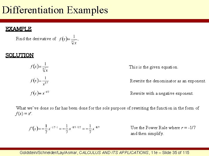
Differentiation Examples EXAMPLE Find the derivative of SOLUTION This is the given equation. Rewrite the denominator as an exponent. Rewrite with a negative exponent. What we’ve done so far has been done for the sole purpose of rewriting the function in the form of f (x) = xr. Use the Power Rule where r = -1/7 and then simplify. Goldstein/Schneider/Lay/Asmar, CALCULUS AND ITS APPLICATIONS, 11 e – Slide 35 of 115

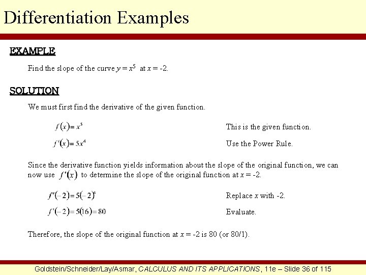
Differentiation Examples EXAMPLE Find the slope of the curve y = x 5 at x = -2. SOLUTION We must first find the derivative of the given function. This is the given function. Use the Power Rule. Since the derivative function yields information about the slope of the original function, we can now use to determine the slope of the original function at x = -2. Replace x with -2. Evaluate. Therefore, the slope of the original function at x = -2 is 80 (or 80/1). Goldstein/Schneider/Lay/Asmar, CALCULUS AND ITS APPLICATIONS, 11 e – Slide 36 of 115

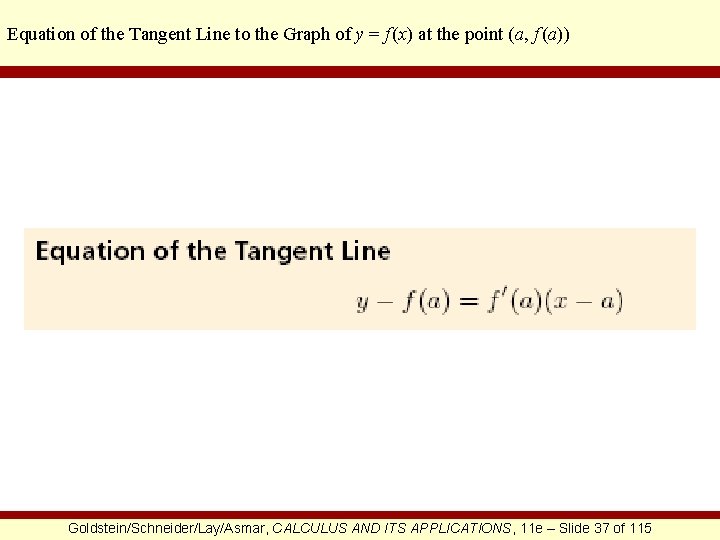
Equation of the Tangent Line to the Graph of y = f (x) at the point (a, f (a)) Goldstein/Schneider/Lay/Asmar, CALCULUS AND ITS APPLICATIONS, 11 e – Slide 37 of 115

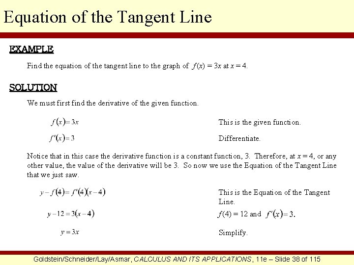
Equation of the Tangent Line EXAMPLE Find the equation of the tangent line to the graph of f (x) = 3 x at x = 4. SOLUTION We must first find the derivative of the given function. This is the given function. Differentiate. Notice that in this case the derivative function is a constant function, 3. Therefore, at x = 4, or any other value, the value of the derivative will be 3. So now we use the Equation of the Tangent Line that we just saw. This is the Equation of the Tangent Line. f (4) = 12 and Simplify. Goldstein/Schneider/Lay/Asmar, CALCULUS AND ITS APPLICATIONS, 11 e – Slide 38 of 115

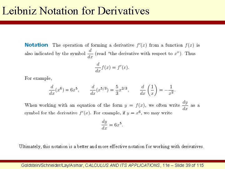
Leibniz Notation for Derivatives Ultimately, this notation is a better and more effective notation for working with derivatives. Goldstein/Schneider/Lay/Asmar, CALCULUS AND ITS APPLICATIONS, 11 e – Slide 39 of 115

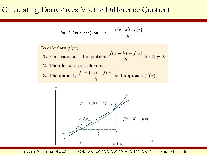
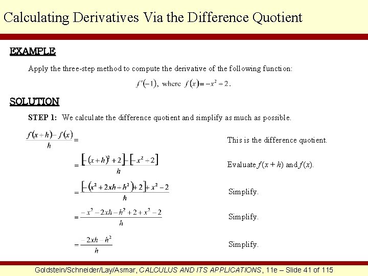
Calculating Derivatives Via the Difference Quotient The Difference Quotient is Goldstein/Schneider/Lay/Asmar, CALCULUS AND ITS APPLICATIONS, 11 e – Slide 40 of 115

Calculating Derivatives Via the Difference Quotient EXAMPLE Apply the three-step method to compute the derivative of the following function: SOLUTION STEP 1: We calculate the difference quotient and simplify as much as possible. This is the difference quotient. Evaluate f (x + h) and f (x). Simplify. Goldstein/Schneider/Lay/Asmar, CALCULUS AND ITS APPLICATIONS, 11 e – Slide 41 of 115

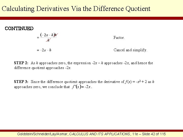
Calculating Derivatives Via the Difference Quotient CONTINUED Factor. Cancel and simplify. STEP 2: As h approaches zero, the expression -2 x – h approaches -2 x, and hence the difference quotient approaches -2 x. STEP 3: Since the difference quotient approaches the derivative of f (x) = -x 2 + 2 as h approaches zero, we conclude that Goldstein/Schneider/Lay/Asmar, CALCULUS AND ITS APPLICATIONS, 11 e – Slide 42 of 115

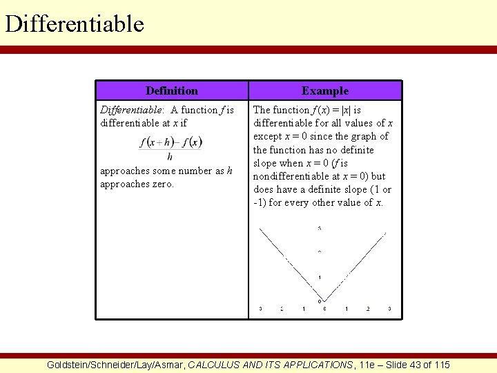
Differentiable Definition Differentiable: A function f is differentiable at x if approaches some number as h approaches zero. Example The function f (x) = |x| is differentiable for all values of x except x = 0 since the graph of the function has no definite slope when x = 0 (f is nondifferentiable at x = 0) but does have a definite slope (1 or -1) for every other value of x. Goldstein/Schneider/Lay/Asmar, CALCULUS AND ITS APPLICATIONS, 11 e – Slide 43 of 115

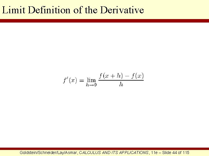
Limit Definition of the Derivative Goldstein/Schneider/Lay/Asmar, CALCULUS AND ITS APPLICATIONS, 11 e – Slide 44 of 115

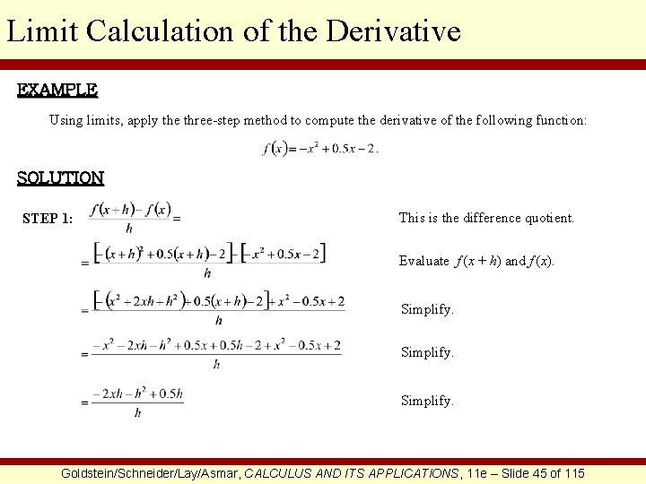
Limit Calculation of the Derivative EXAMPLE Using limits, apply the three-step method to compute the derivative of the following function: SOLUTION STEP 1: This is the difference quotient. Evaluate f (x + h) and f (x). Simplify. Goldstein/Schneider/Lay/Asmar, CALCULUS AND ITS APPLICATIONS, 11 e – Slide 45 of 115

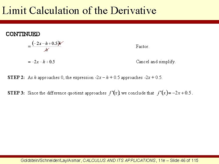
Limit Calculation of the Derivative CONTINUED Factor. Cancel and simplify. STEP 2: As h approaches 0, the expression -2 x – h + 0. 5 approaches -2 x + 0. 5. STEP 3: Since the difference quotient approaches , we conclude that Goldstein/Schneider/Lay/Asmar, CALCULUS AND ITS APPLICATIONS, 11 e – Slide 46 of 115

§ 1. 4 Limits and the Derivative Goldstein/Schneider/Lay/Asmar, CALCULUS AND ITS APPLICATIONS, 11 e – Slide 47 of 115

Section Outline q Definition of the Limit q Finding Limits q Limit Theorems q Using Limits to Calculate a Derivative q Limits as x Increases Without Bound Goldstein/Schneider/Lay/Asmar, CALCULUS AND ITS APPLICATIONS, 11 e – Slide 48 of 115

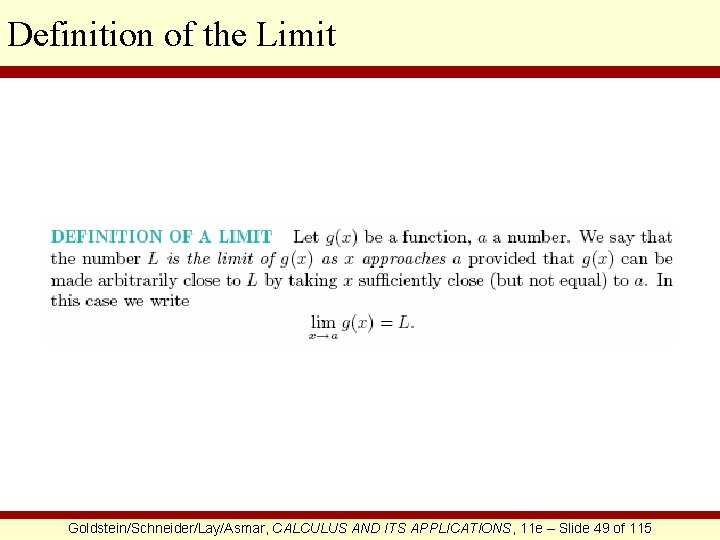
Definition of the Limit Goldstein/Schneider/Lay/Asmar, CALCULUS AND ITS APPLICATIONS, 11 e – Slide 49 of 115

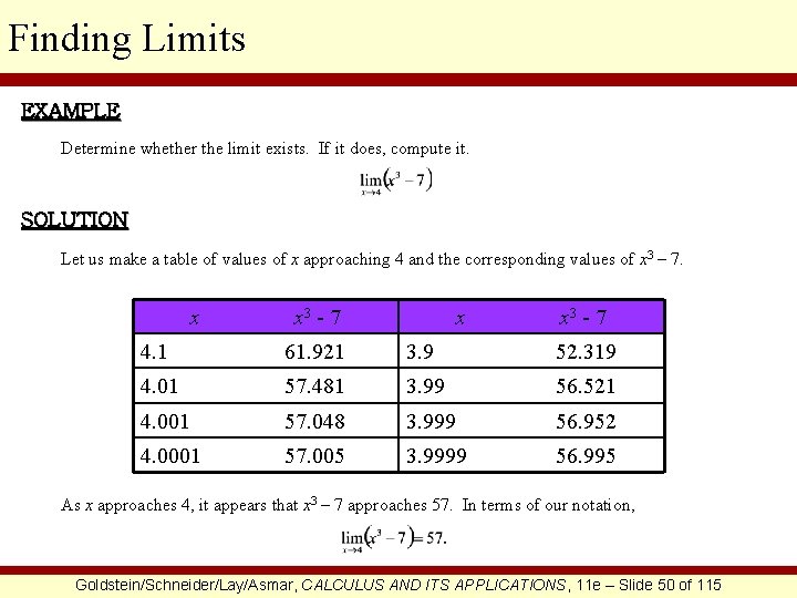
Finding Limits EXAMPLE Determine whether the limit exists. If it does, compute it. SOLUTION Let us make a table of values of x approaching 4 and the corresponding values of x 3 – 7. x x 3 - 7 4. 1 61. 921 3. 9 52. 319 4. 01 57. 481 3. 99 56. 521 4. 001 57. 048 3. 999 56. 952 4. 0001 57. 005 3. 9999 56. 995 As x approaches 4, it appears that x 3 – 7 approaches 57. In terms of our notation, Goldstein/Schneider/Lay/Asmar, CALCULUS AND ITS APPLICATIONS, 11 e – Slide 50 of 115

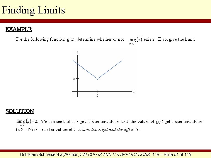
Finding Limits EXAMPLE For the following function g(x), determine whether or not exists. If so, give the limit. SOLUTION We can see that as x gets closer and closer to 3, the values of g(x) get closer and closer to 2. This is true for values of x to both the right and the left of 3. Goldstein/Schneider/Lay/Asmar, CALCULUS AND ITS APPLICATIONS, 11 e – Slide 51 of 115

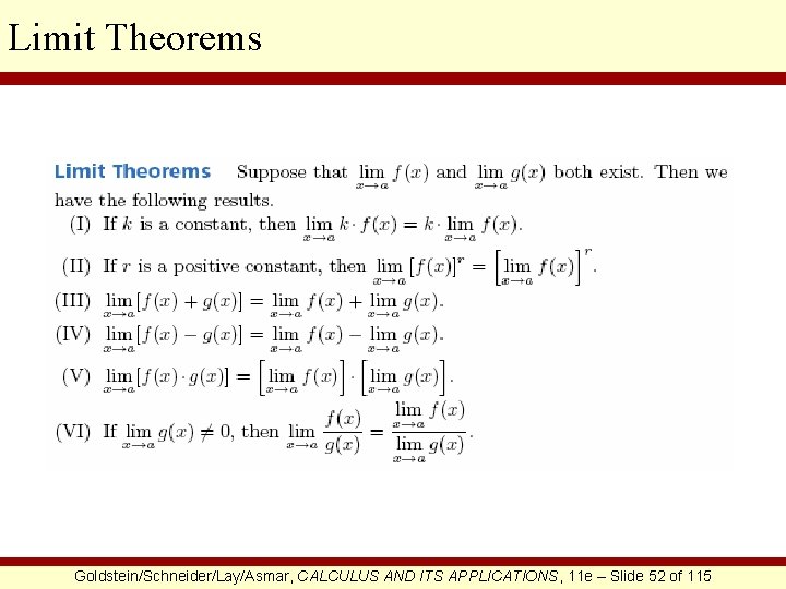
Limit Theorems Goldstein/Schneider/Lay/Asmar, CALCULUS AND ITS APPLICATIONS, 11 e – Slide 52 of 115

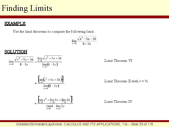
Finding Limits EXAMPLE Use the limit theorems to compute the following limit. SOLUTION Limit Theorem VI Limit Theorem II with r = ½ Limit Theorem IV Goldstein/Schneider/Lay/Asmar, CALCULUS AND ITS APPLICATIONS, 11 e – Slide 53 of 115

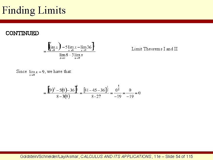
Finding Limits CONTINUED Limit Theorems I and II Since , we have that: Goldstein/Schneider/Lay/Asmar, CALCULUS AND ITS APPLICATIONS, 11 e – Slide 54 of 115

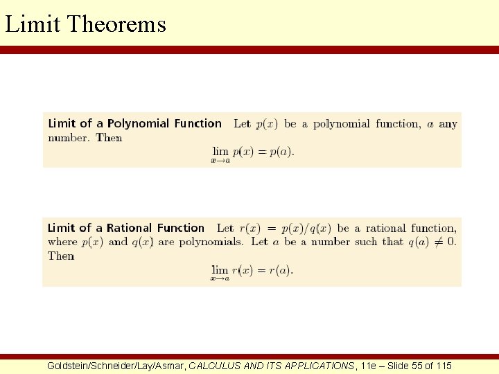
Limit Theorems Goldstein/Schneider/Lay/Asmar, CALCULUS AND ITS APPLICATIONS, 11 e – Slide 55 of 115

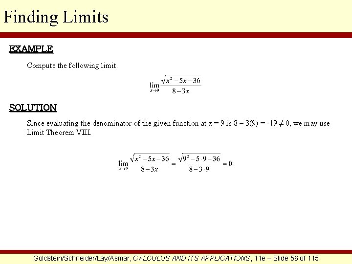
Finding Limits EXAMPLE Compute the following limit. SOLUTION Since evaluating the denominator of the given function at x = 9 is 8 – 3(9) = -19 ≠ 0, we may use Limit Theorem VIII. Goldstein/Schneider/Lay/Asmar, CALCULUS AND ITS APPLICATIONS, 11 e – Slide 56 of 115

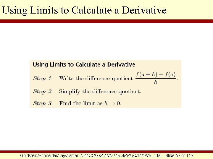
Using Limits to Calculate a Derivative Goldstein/Schneider/Lay/Asmar, CALCULUS AND ITS APPLICATIONS, 11 e – Slide 57 of 115

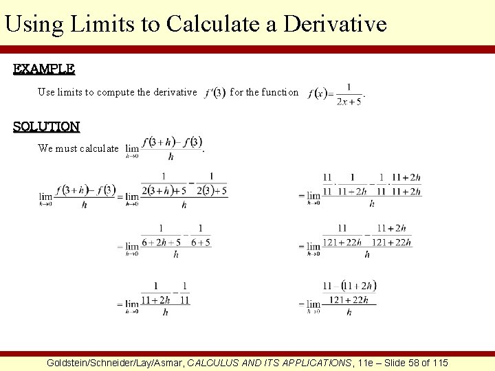
Using Limits to Calculate a Derivative EXAMPLE Use limits to compute the derivative for the function SOLUTION We must calculate Goldstein/Schneider/Lay/Asmar, CALCULUS AND ITS APPLICATIONS, 11 e – Slide 58 of 115

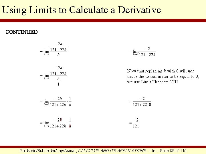
Using Limits to Calculate a Derivative CONTINUED Now that replacing h with 0 will not cause the denominator to be equal to 0, we use Limit Theorem VIII. Goldstein/Schneider/Lay/Asmar, CALCULUS AND ITS APPLICATIONS, 11 e – Slide 59 of 115

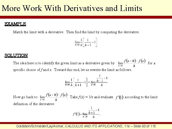
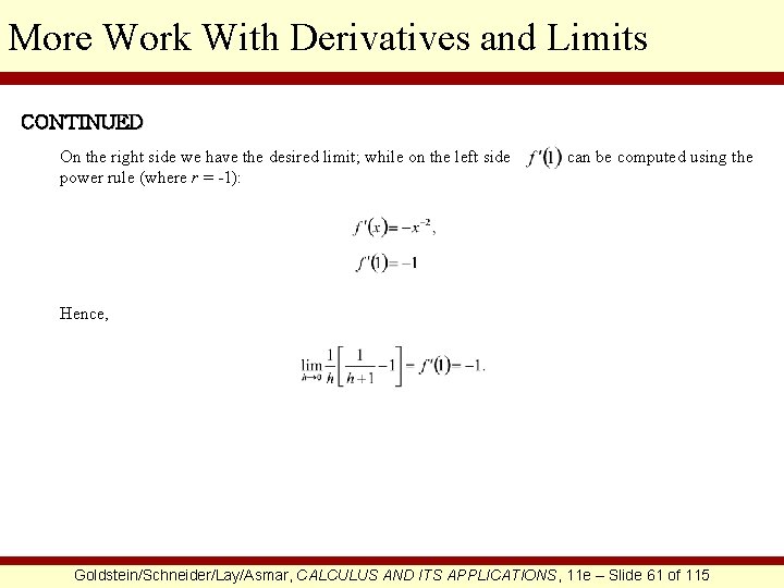
More Work With Derivatives and Limits EXAMPLE Match the limit with a derivative. Then find the limit by computing the derivative. SOLUTION The idea here is to identify the given limit as a derivative given by for a specific choice of f and x. Toward this end, let us rewrite the limit as follows. Now go back to . Take f (x) = 1/x and evaluate according to the limit definition of the derivative: Goldstein/Schneider/Lay/Asmar, CALCULUS AND ITS APPLICATIONS, 11 e – Slide 60 of 115

More Work With Derivatives and Limits CONTINUED On the right side we have the desired limit; while on the left side power rule (where r = -1): can be computed using the Hence, Goldstein/Schneider/Lay/Asmar, CALCULUS AND ITS APPLICATIONS, 11 e – Slide 61 of 115

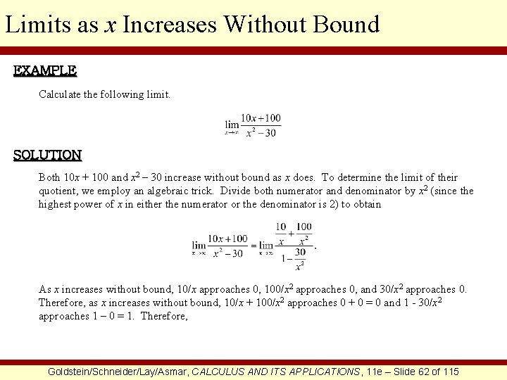
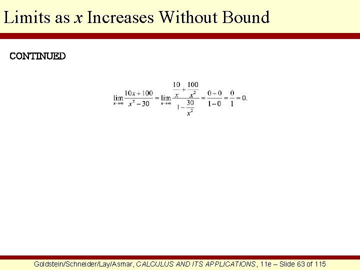
Limits as x Increases Without Bound EXAMPLE Calculate the following limit. SOLUTION Both 10 x + 100 and x 2 – 30 increase without bound as x does. To determine the limit of their quotient, we employ an algebraic trick. Divide both numerator and denominator by x 2 (since the highest power of x in either the numerator or the denominator is 2) to obtain As x increases without bound, 10/x approaches 0, 100/x 2 approaches 0, and 30/x 2 approaches 0. Therefore, as x increases without bound, 10/x + 100/x 2 approaches 0 + 0 = 0 and 1 - 30/x 2 approaches 1 – 0 = 1. Therefore, Goldstein/Schneider/Lay/Asmar, CALCULUS AND ITS APPLICATIONS, 11 e – Slide 62 of 115

Limits as x Increases Without Bound CONTINUED Goldstein/Schneider/Lay/Asmar, CALCULUS AND ITS APPLICATIONS, 11 e – Slide 63 of 115

§ 1. 5 Differentiability and Continuity Goldstein/Schneider/Lay/Asmar, CALCULUS AND ITS APPLICATIONS, 11 e – Slide 64 of 115

Section Outline q Differentiability and Nondifferentiability q Graphs Nondifferentiable at a Point q Continuous and Discontinuous Functions Goldstein/Schneider/Lay/Asmar, CALCULUS AND ITS APPLICATIONS, 11 e – Slide 65 of 115

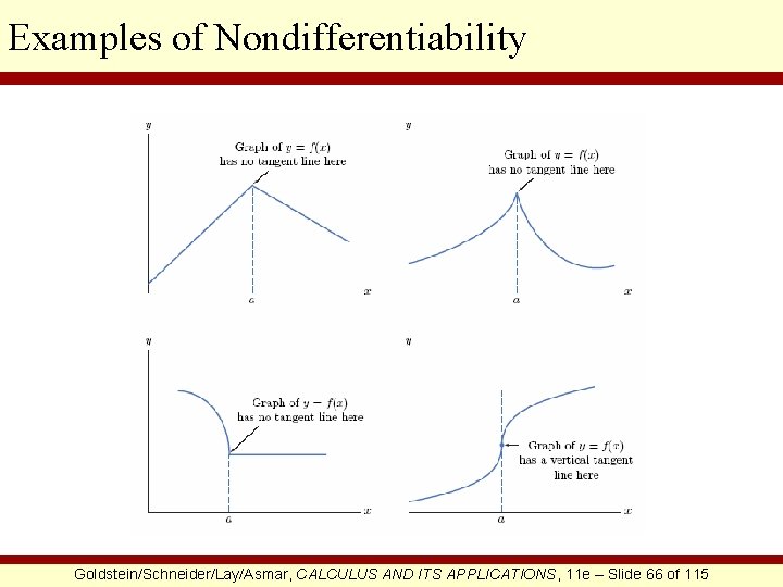
Examples of Nondifferentiability Goldstein/Schneider/Lay/Asmar, CALCULUS AND ITS APPLICATIONS, 11 e – Slide 66 of 115

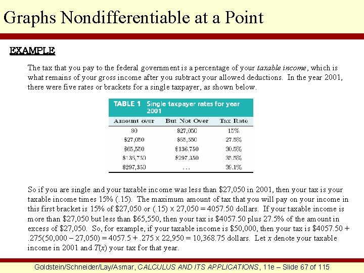
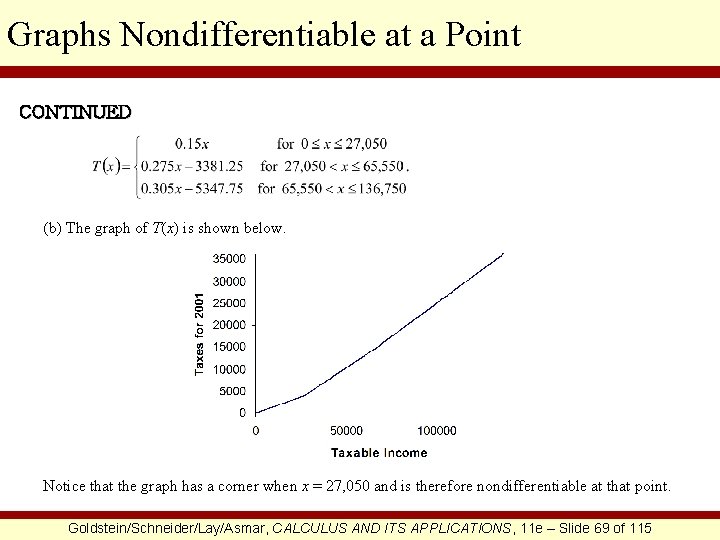
Graphs Nondifferentiable at a Point EXAMPLE The tax that you pay to the federal government is a percentage of your taxable income, which is what remains of your gross income after you subtract your allowed deductions. In the year 2001, there were five rates or brackets for a single taxpayer, as shown below. So if you are single and your taxable income was less than $27, 050 in 2001, then your tax is your taxable income times 15% (. 15). The maximum amount of tax that you will pay on your income in this first bracket is 15% of $27, 050 or (. 15) x 27, 050 = 4057. 50 dollars. If your taxable income is more than $27, 050 but less than $65, 550, then your tax is $4057. 50 plus 27. 5% of the amount in excess of $27, 050. So, for example, if your taxable income is $50, 000, then your tax is $4057. 50 +. 275(50, 000 – 27, 050) = 4057. 5 +. 275 x 22, 950 = 10, 368. 75 dollars. Let x denote your taxable income in 2001 and T(x) your tax for that year. Goldstein/Schneider/Lay/Asmar, CALCULUS AND ITS APPLICATIONS, 11 e – Slide 67 of 115

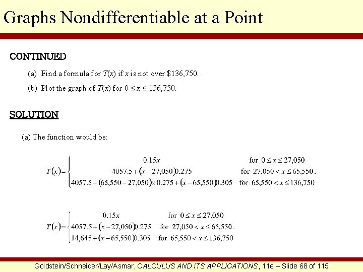
Graphs Nondifferentiable at a Point CONTINUED (a) Find a formula for T(x) if x is not over $136, 750. (b) Plot the graph of T(x) for 0 ≤ x ≤ 136, 750. SOLUTION (a) The function would be: Goldstein/Schneider/Lay/Asmar, CALCULUS AND ITS APPLICATIONS, 11 e – Slide 68 of 115

Graphs Nondifferentiable at a Point CONTINUED (b) The graph of T(x) is shown below. Notice that the graph has a corner when x = 27, 050 and is therefore nondifferentiable at that point. Goldstein/Schneider/Lay/Asmar, CALCULUS AND ITS APPLICATIONS, 11 e – Slide 69 of 115

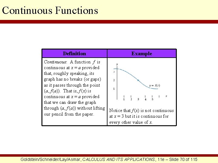
Continuous Functions Definition Example Continuous: A function f is continuous at x = a provided that, roughly speaking, its graph has no breaks (or gaps) as it passes through the point (a, f (a)). That is, f (x) is continuous at x = a provided that we can draw the graph through (a, f (a)) without lifting Notice that f (x) is not continuous our pencil from the paper. at x = 3 but it is continuous for every other value of x. Goldstein/Schneider/Lay/Asmar, CALCULUS AND ITS APPLICATIONS, 11 e – Slide 70 of 115

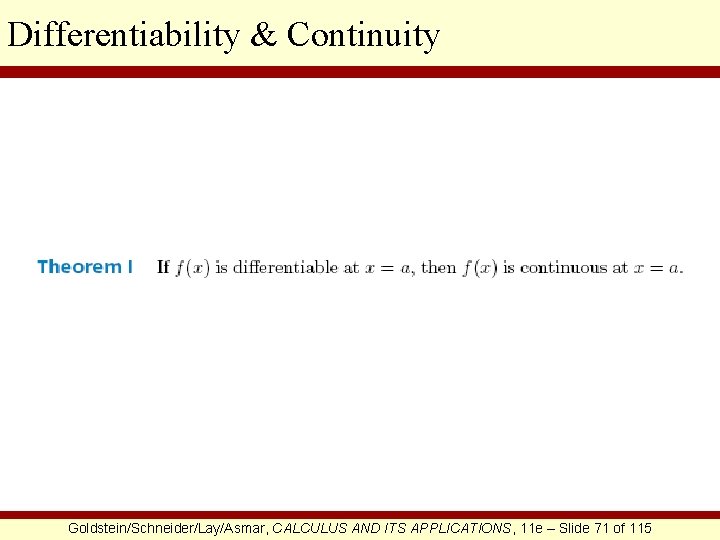
Differentiability & Continuity Goldstein/Schneider/Lay/Asmar, CALCULUS AND ITS APPLICATIONS, 11 e – Slide 71 of 115

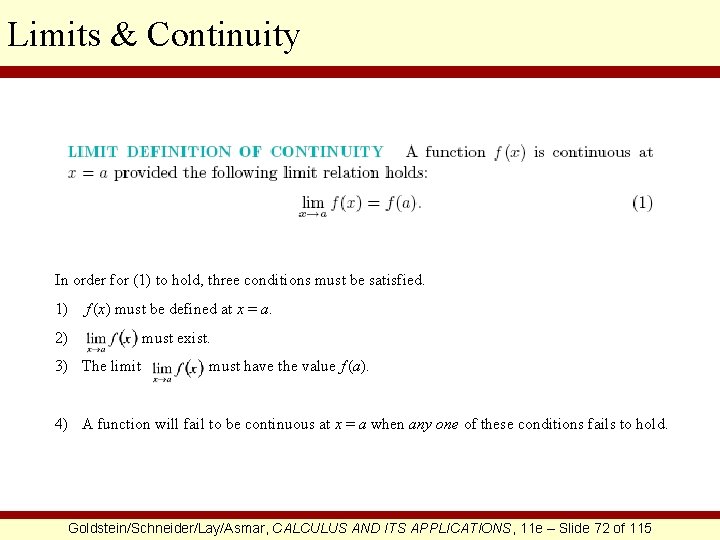
Limits & Continuity In order for (1) to hold, three conditions must be satisfied. 1) f (x) must be defined at x = a. 2) must exist. 3) The limit must have the value f (a). 4) A function will fail to be continuous at x = a when any one of these conditions fails to hold. Goldstein/Schneider/Lay/Asmar, CALCULUS AND ITS APPLICATIONS, 11 e – Slide 72 of 115

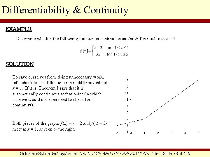
Differentiability & Continuity EXAMPLE Determine whether the following function is continuous and/or differentiable at x = 1. SOLUTION To save ourselves from doing unnecessary work, let’s check to see if the function is differentiable at x = 1. If it is, Theorem I says that it is automatically continuous at that point (in which case we would not even need to check for continuity). Both pieces of the graph, f (x) = x + 2 and f (x) = 3 x meet at x = 1, as seen to the right. Goldstein/Schneider/Lay/Asmar, CALCULUS AND ITS APPLICATIONS, 11 e – Slide 73 of 115

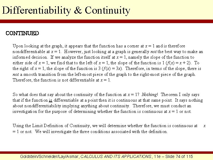
Differentiability & Continuity CONTINUED Upon looking at the graph, it appears that the function has a corner at x = 1 and is therefore nondifferentiable at x = 1. However, just looking at a graph is generally not the best way to make an informed decision. If we analyze the function itself at x = 1, namely the slope of the function to either side of x = 1, we find that to the left of x = 1, the slope of the function is 1 (f (x) = x + 2). To the right of x = 1, the slope of the function is 3 (f (x) = 3 x). Therefore, in terms of the slope, there is not a smooth transition from the left-most piece of the graph to the right-most piece of the graph. Therefore, the function is not differentiable at x = 1. So what does that say about the continuity of the function at x = 1? Nothing! Theorem I only says that if the function is differentiable at a point then it is continuous at that same point. It says nothing about nondifferentiability implying anything about continuity. Therefore, we must conduct an investigation for the purpose of determining whether the function is continuous at x = 1 or not. Using the Limit Definition of Continuity, we will determine whether the function is continuous at = 1 or not. We will investigate three conditions associated with the definition. Goldstein/Schneider/Lay/Asmar, CALCULUS AND ITS APPLICATIONS, 11 e – Slide 74 of 115 x

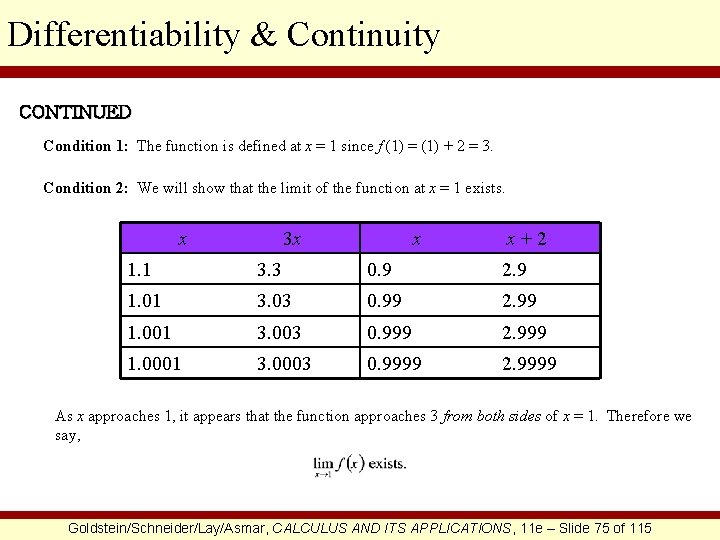
Differentiability & Continuity CONTINUED Condition 1: The function is defined at x = 1 since f (1) = (1) + 2 = 3. Condition 2: We will show that the limit of the function at x = 1 exists. x 3 x x x+2 1. 1 3. 3 0. 9 2. 9 1. 01 3. 03 0. 99 2. 99 1. 001 3. 003 0. 999 2. 999 1. 0001 3. 0003 0. 9999 2. 9999 As x approaches 1, it appears that the function approaches 3 from both sides of x = 1. Therefore we say, Goldstein/Schneider/Lay/Asmar, CALCULUS AND ITS APPLICATIONS, 11 e – Slide 75 of 115

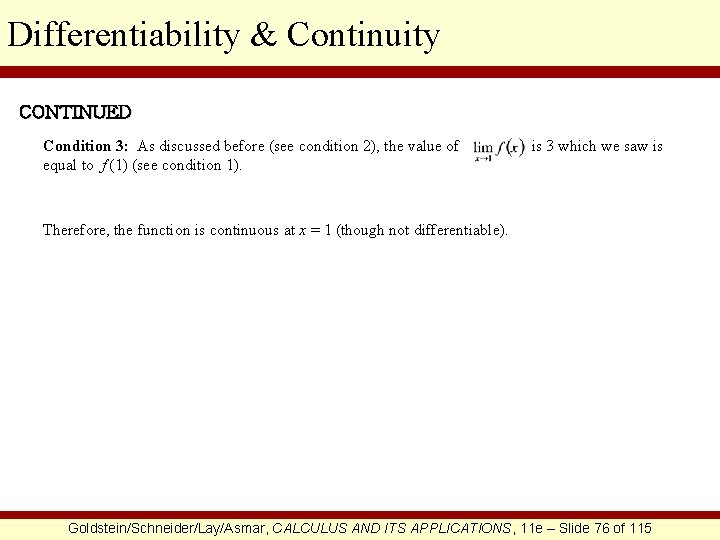
Differentiability & Continuity CONTINUED Condition 3: As discussed before (see condition 2), the value of equal to f (1) (see condition 1). is 3 which we saw is Therefore, the function is continuous at x = 1 (though not differentiable). Goldstein/Schneider/Lay/Asmar, CALCULUS AND ITS APPLICATIONS, 11 e – Slide 76 of 115

§ 1. 6 Some Rules for Differentiation Goldstein/Schneider/Lay/Asmar, CALCULUS AND ITS APPLICATIONS, 11 e – Slide 77 of 115

Section Outline q Some Rules of Differentiation q The Derivative as a Rate of Change Goldstein/Schneider/Lay/Asmar, CALCULUS AND ITS APPLICATIONS, 11 e – Slide 78 of 115

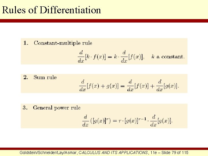
Rules of Differentiation Goldstein/Schneider/Lay/Asmar, CALCULUS AND ITS APPLICATIONS, 11 e – Slide 79 of 115

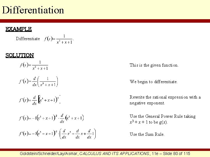
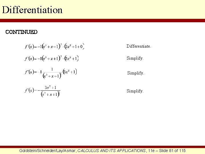
Differentiation EXAMPLE Differentiate SOLUTION This is the given function. We begin to differentiate. Rewrite the rational expression with a negative exponent. Use the General Power Rule taking x 3 + x + 1 to be g(x). Use the Sum Rule. Goldstein/Schneider/Lay/Asmar, CALCULUS AND ITS APPLICATIONS, 11 e – Slide 80 of 115

Differentiation CONTINUED Differentiate. Simplify. Goldstein/Schneider/Lay/Asmar, CALCULUS AND ITS APPLICATIONS, 11 e – Slide 81 of 115

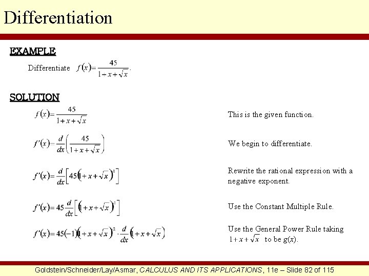
Differentiation EXAMPLE Differentiate SOLUTION This is the given function. We begin to differentiate. Rewrite the rational expression with a negative exponent. Use the Constant Multiple Rule. Use the General Power Rule taking to be g(x). Goldstein/Schneider/Lay/Asmar, CALCULUS AND ITS APPLICATIONS, 11 e – Slide 82 of 115

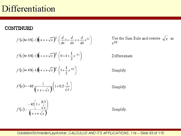
Differentiation CONTINUED Use the Sum Rule and rewrite x 1/2. Differentiate. Simplify. Goldstein/Schneider/Lay/Asmar, CALCULUS AND ITS APPLICATIONS, 11 e – Slide 83 of 115 as

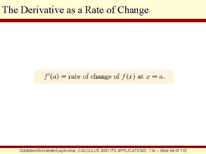
The Derivative as a Rate of Change Goldstein/Schneider/Lay/Asmar, CALCULUS AND ITS APPLICATIONS, 11 e – Slide 84 of 115

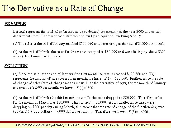
The Derivative as a Rate of Change EXAMPLE Let S(x) represent the total sales (in thousands of dollars) for month x in the year 2005 at a certain department store. Represent each statement below by an equation involving S or. (a) The sales at the end of January reached $120, 560 and were rising at the rate of $1500 per month. (b) At the end of March, the sales for this month dropped to $80, 000 and were falling by about $200 a day (Use 1 month = 30 days). SOLUTION (a) Since the sales at the end of January (the first month, so x = 1) reached $120, 560 and S(x) represents the amount of sales for a given month, we have: S(1) = 120, 560. Further, since the rate of change of sales (rate of change means we will use the derivative of S(x)) for the month of January is a positive $1500 per month, we have: (b) At the end of March (the third month, so x = 3), the sales dropped to $80, 000. Therefore, sales for the month of March was $80, 000. That is: S(3) = 80, 000. Additionally, since sales were dropping by $200 per day during March, this means that the rate of change of the function S(x) was (30 days) x (-200 dollars) = -6000 dollars per month. Therefore, we have: Goldstein/Schneider/Lay/Asmar, CALCULUS AND ITS APPLICATIONS, 11 e – Slide 85 of 115

§ 1. 7 More About Derivatives Goldstein/Schneider/Lay/Asmar, CALCULUS AND ITS APPLICATIONS, 11 e – Slide 86 of 115

Section Outline q Differentiating Various Independent Variables q Computing Second Derivatives q Second Derivatives Evaluated at a Point q Marginal Cost q Marginal Revenue q Marginal Profit Goldstein/Schneider/Lay/Asmar, CALCULUS AND ITS APPLICATIONS, 11 e – Slide 87 of 115

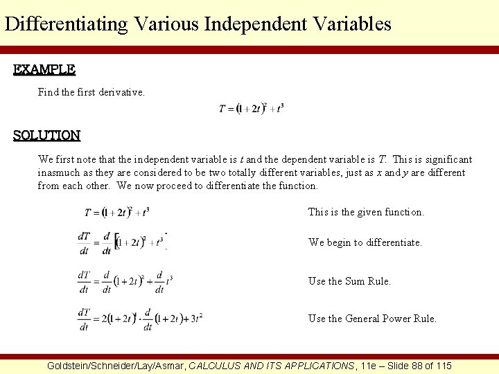
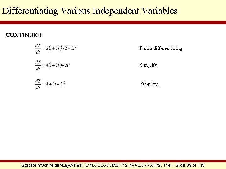
Differentiating Various Independent Variables EXAMPLE Find the first derivative. SOLUTION We first note that the independent variable is t and the dependent variable is T. This is significant inasmuch as they are considered to be two totally different variables, just as x and y are different from each other. We now proceed to differentiate the function. This is the given function. We begin to differentiate. Use the Sum Rule. Use the General Power Rule. Goldstein/Schneider/Lay/Asmar, CALCULUS AND ITS APPLICATIONS, 11 e – Slide 88 of 115

Differentiating Various Independent Variables CONTINUED Finish differentiating. Simplify. Goldstein/Schneider/Lay/Asmar, CALCULUS AND ITS APPLICATIONS, 11 e – Slide 89 of 115

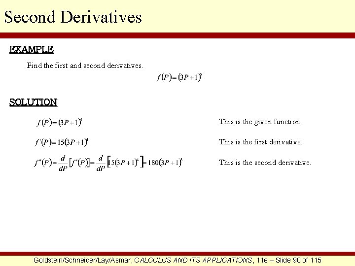
Second Derivatives EXAMPLE Find the first and second derivatives. SOLUTION This is the given function. This is the first derivative. This is the second derivative. Goldstein/Schneider/Lay/Asmar, CALCULUS AND ITS APPLICATIONS, 11 e – Slide 90 of 115

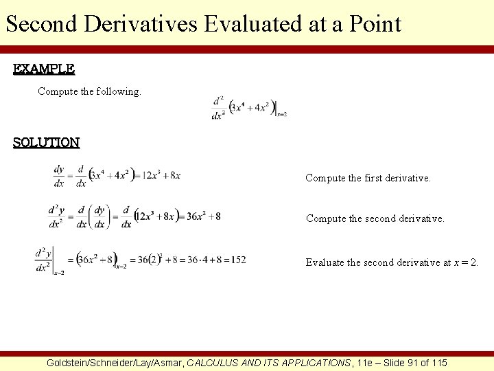
Second Derivatives Evaluated at a Point EXAMPLE Compute the following. SOLUTION Compute the first derivative. Compute the second derivative. Evaluate the second derivative at x = 2. Goldstein/Schneider/Lay/Asmar, CALCULUS AND ITS APPLICATIONS, 11 e – Slide 91 of 115

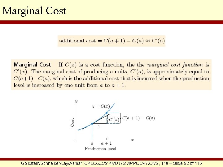
Marginal Cost Goldstein/Schneider/Lay/Asmar, CALCULUS AND ITS APPLICATIONS, 11 e – Slide 92 of 115

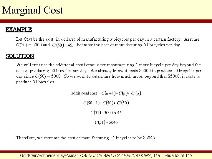
Marginal Cost EXAMPLE Let C(x) be the cost (in dollars) of manufacturing x bicycles per day in a certain factory. Assume C(50) = 5000 and Estimate the cost of manufacturing 51 bicycles per day. SOLUTION We will first use the additional cost formula for manufacturing 1 more bicycle per day beyond the cost of producing 50 bicycles per day. We already know it costs $5000 to produce 50 bicycles per day since C(50) = 5000. So we wish to determine how much more, beyond that $5000, it costs to produce 51 bicycles. Therefore, we estimate the cost of manufacturing 51 bicycles to be $5045. Goldstein/Schneider/Lay/Asmar, CALCULUS AND ITS APPLICATIONS, 11 e – Slide 93 of 115

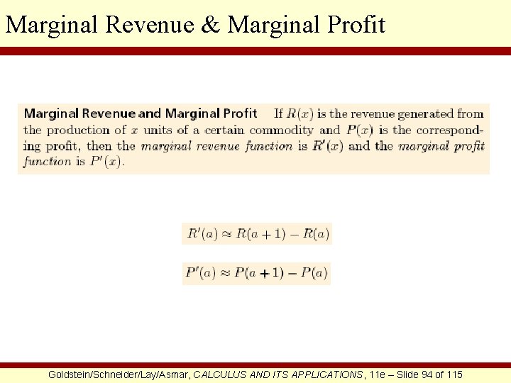
Marginal Revenue & Marginal Profit Goldstein/Schneider/Lay/Asmar, CALCULUS AND ITS APPLICATIONS, 11 e – Slide 94 of 115

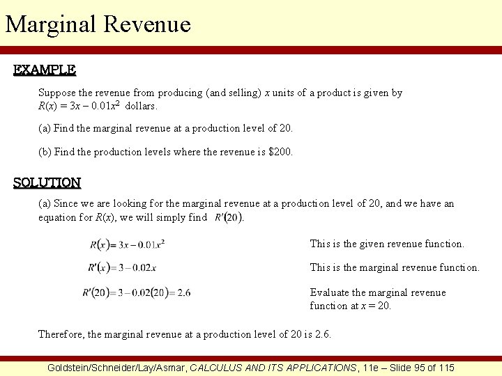
Marginal Revenue EXAMPLE Suppose the revenue from producing (and selling) x units of a product is given by R(x) = 3 x – 0. 01 x 2 dollars. (a) Find the marginal revenue at a production level of 20. (b) Find the production levels where the revenue is $200. SOLUTION (a) Since we are looking for the marginal revenue at a production level of 20, and we have an equation for R(x), we will simply find This is the given revenue function. This is the marginal revenue function. Evaluate the marginal revenue function at x = 20. Therefore, the marginal revenue at a production level of 20 is 2. 6. Goldstein/Schneider/Lay/Asmar, CALCULUS AND ITS APPLICATIONS, 11 e – Slide 95 of 115

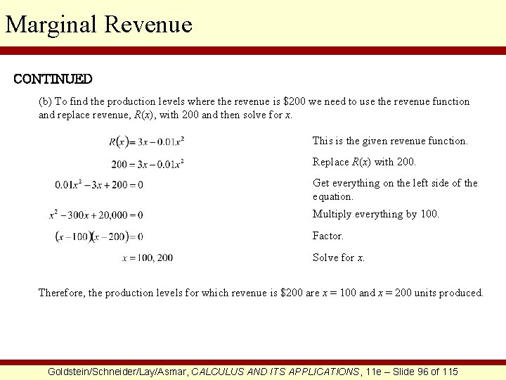
Marginal Revenue CONTINUED (b) To find the production levels where the revenue is $200 we need to use the revenue function and replace revenue, R(x), with 200 and then solve for x. This is the given revenue function. Replace R(x) with 200. Get everything on the left side of the equation. Multiply everything by 100. Factor. Solve for x. Therefore, the production levels for which revenue is $200 are x = 100 and x = 200 units produced. Goldstein/Schneider/Lay/Asmar, CALCULUS AND ITS APPLICATIONS, 11 e – Slide 96 of 115

§ 1. 8 The Derivative as a Rate of Change Goldstein/Schneider/Lay/Asmar, CALCULUS AND ITS APPLICATIONS, 11 e – Slide 97 of 115

Section Outline q Average Rate of Change q Instantaneous Rate of Change q Average Velocity q Position, Velocity, and Acceleration q Approximating the Change in a Function Goldstein/Schneider/Lay/Asmar, CALCULUS AND ITS APPLICATIONS, 11 e – Slide 98 of 115

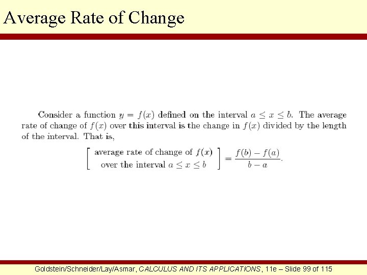
Average Rate of Change Goldstein/Schneider/Lay/Asmar, CALCULUS AND ITS APPLICATIONS, 11 e – Slide 99 of 115

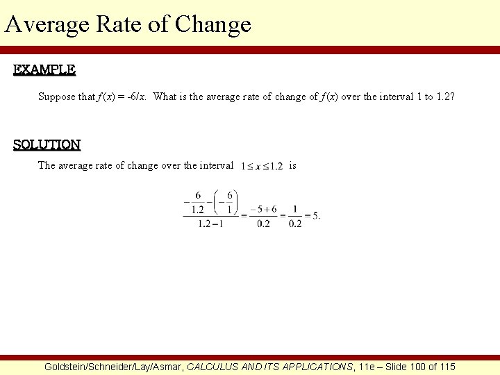
Average Rate of Change EXAMPLE Suppose that f (x) = -6/x. What is the average rate of change of f (x) over the interval 1 to 1. 2? SOLUTION The average rate of change over the interval is Goldstein/Schneider/Lay/Asmar, CALCULUS AND ITS APPLICATIONS, 11 e – Slide 100 of 115

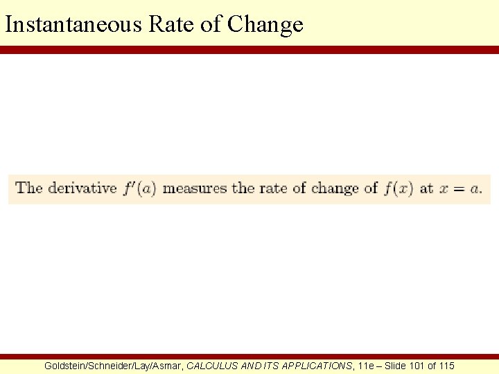
Instantaneous Rate of Change Goldstein/Schneider/Lay/Asmar, CALCULUS AND ITS APPLICATIONS, 11 e – Slide 101 of 115

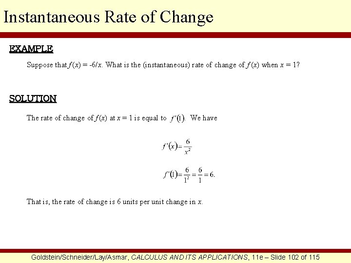
Instantaneous Rate of Change EXAMPLE Suppose that f (x) = -6/x. What is the (instantaneous) rate of change of f (x) when x = 1? SOLUTION The rate of change of f (x) at x = 1 is equal to . We have That is, the rate of change is 6 units per unit change in x. Goldstein/Schneider/Lay/Asmar, CALCULUS AND ITS APPLICATIONS, 11 e – Slide 102 of 115

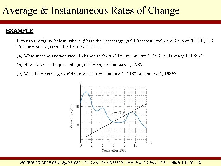
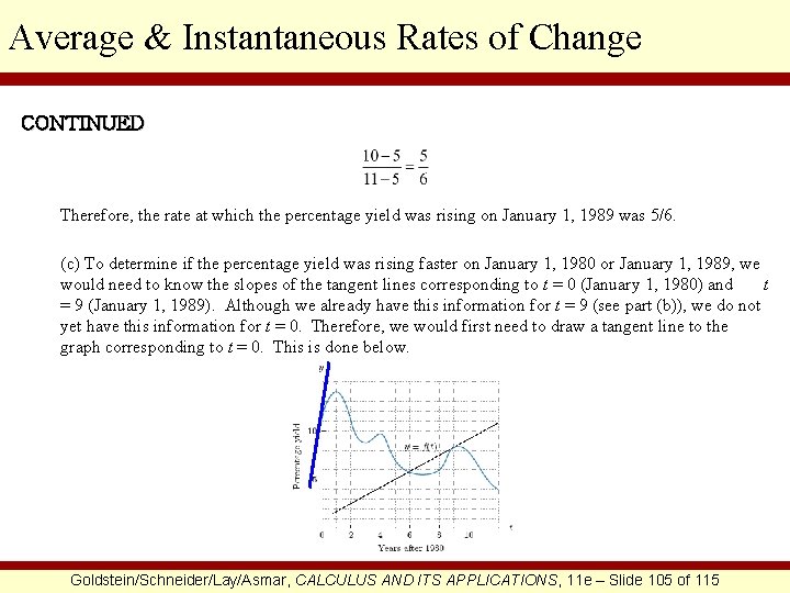
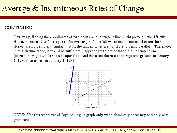
Average & Instantaneous Rates of Change EXAMPLE Refer to the figure below, where f (t) is the percentage yield (interest rate) on a 3 -month T-bill (U. S. Treasury bill) t years after January 1, 1980. (a) What was the average rate of change in the yield from January 1, 1981 to January 1, 1985? (b) How fast was the percentage yield rising on January 1, 1989? (c) Was the percentage yield rising faster on January 1, 1980 or January 1, 1989? Goldstein/Schneider/Lay/Asmar, CALCULUS AND ITS APPLICATIONS, 11 e – Slide 103 of 115

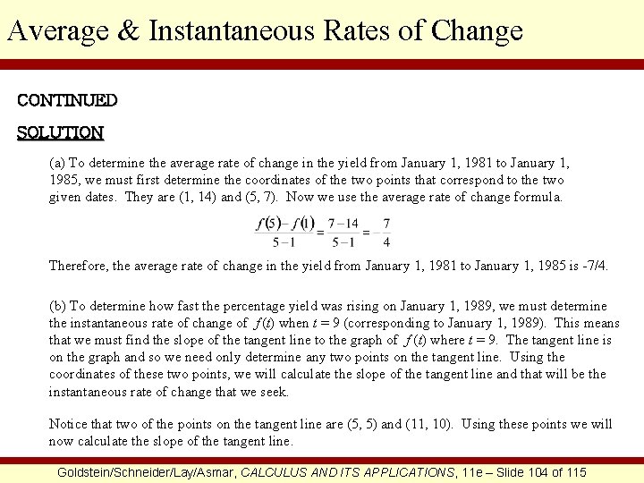
Average & Instantaneous Rates of Change CONTINUED SOLUTION (a) To determine the average rate of change in the yield from January 1, 1981 to January 1, 1985, we must first determine the coordinates of the two points that correspond to the two given dates. They are (1, 14) and (5, 7). Now we use the average rate of change formula. Therefore, the average rate of change in the yield from January 1, 1981 to January 1, 1985 is -7/4. (b) To determine how fast the percentage yield was rising on January 1, 1989, we must determine the instantaneous rate of change of f (t) when t = 9 (corresponding to January 1, 1989). This means that we must find the slope of the tangent line to the graph of f (t) where t = 9. The tangent line is on the graph and so we need only determine any two points on the tangent line. Using the coordinates of these two points, we will calculate the slope of the tangent line and that will be the instantaneous rate of change that we seek. Notice that two of the points on the tangent line are (5, 5) and (11, 10). Using these points we will now calculate the slope of the tangent line. Goldstein/Schneider/Lay/Asmar, CALCULUS AND ITS APPLICATIONS, 11 e – Slide 104 of 115

Average & Instantaneous Rates of Change CONTINUED Therefore, the rate at which the percentage yield was rising on January 1, 1989 was 5/6. (c) To determine if the percentage yield was rising faster on January 1, 1980 or January 1, 1989, we would need to know the slopes of the tangent lines corresponding to t = 0 (January 1, 1980) and t = 9 (January 1, 1989). Although we already have this information for t = 9 (see part (b)), we do not yet have this information for t = 0. Therefore, we would first need to draw a tangent line to the graph corresponding to t = 0. This is done below. Goldstein/Schneider/Lay/Asmar, CALCULUS AND ITS APPLICATIONS, 11 e – Slide 105 of 115

Average & Instantaneous Rates of Change CONTINUED Obviously, finding the coordinates of two points on this tangent line might prove a little difficult. However, notice that the slopes of the two tangent lines (all we’re really interested in are their slopes) are not remotely similar (that is, the tangent lines are not close to being parallel). Therefore, in this circumstance, it would be sufficiently appropriate to notice that the blue tangent line (corresponding to t = 0) has a steeper slope and therefore the rate of change was greater on January 1, 1980 than it was on January 1, 1989. NOTE: Use this technique of “eye-balling” a graph only when absolutely necessary and only with great care. Goldstein/Schneider/Lay/Asmar, CALCULUS AND ITS APPLICATIONS, 11 e – Slide 106 of 115

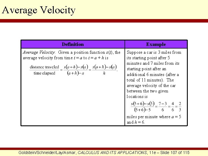
Average Velocity Definition Average Velocity: Given a position function s(t), the average velocity from time t = a to t = a + h is Example Suppose a car is 3 miles from its starting point after 5 minutes and 7 miles from its starting point after an additional 6 minutes (after a total of 11 minutes). The average velocity of the car between the two given locations is miles per minute where a = 5 and h = 6. Goldstein/Schneider/Lay/Asmar, CALCULUS AND ITS APPLICATIONS, 11 e – Slide 107 of 115

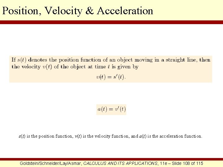
Position, Velocity & Acceleration s(t) is the position function, v(t) is the velocity function, and a(t) is the acceleration function. Goldstein/Schneider/Lay/Asmar, CALCULUS AND ITS APPLICATIONS, 11 e – Slide 108 of 115

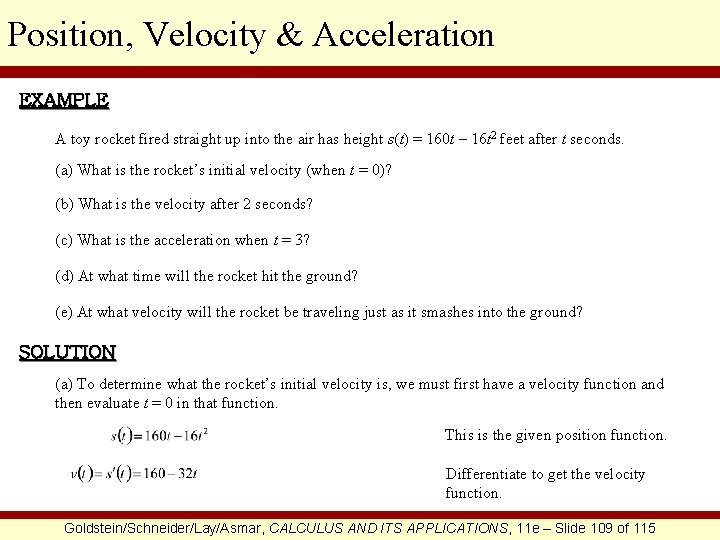
Position, Velocity & Acceleration EXAMPLE A toy rocket fired straight up into the air has height s(t) = 160 t – 16 t 2 feet after t seconds. (a) What is the rocket’s initial velocity (when t = 0)? (b) What is the velocity after 2 seconds? (c) What is the acceleration when t = 3? (d) At what time will the rocket hit the ground? (e) At what velocity will the rocket be traveling just as it smashes into the ground? SOLUTION (a) To determine what the rocket’s initial velocity is, we must first have a velocity function and then evaluate t = 0 in that function. This is the given position function. Differentiate to get the velocity function. Goldstein/Schneider/Lay/Asmar, CALCULUS AND ITS APPLICATIONS, 11 e – Slide 109 of 115

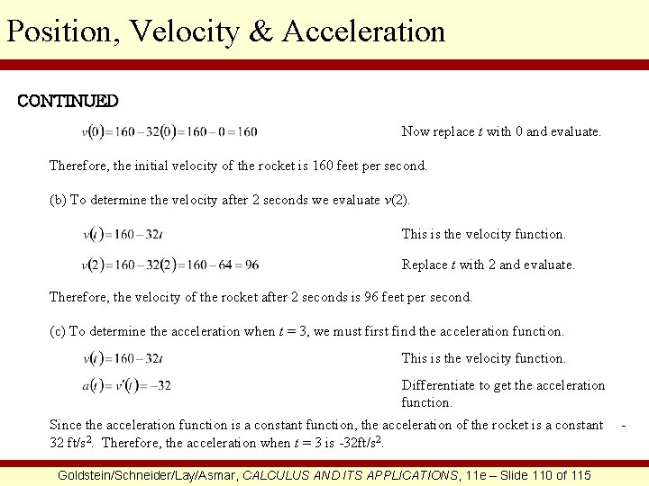
Position, Velocity & Acceleration CONTINUED Now replace t with 0 and evaluate. Therefore, the initial velocity of the rocket is 160 feet per second. (b) To determine the velocity after 2 seconds we evaluate v(2). This is the velocity function. Replace t with 2 and evaluate. Therefore, the velocity of the rocket after 2 seconds is 96 feet per second. (c) To determine the acceleration when t = 3, we must first find the acceleration function. This is the velocity function. Differentiate to get the acceleration function. Since the acceleration function is a constant function, the acceleration of the rocket is a constant 32 ft/s 2. Therefore, the acceleration when t = 3 is -32 ft/s 2. Goldstein/Schneider/Lay/Asmar, CALCULUS AND ITS APPLICATIONS, 11 e – Slide 110 of 115 -

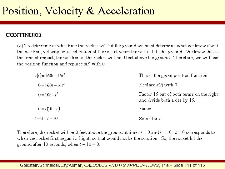
Position, Velocity & Acceleration CONTINUED (d) To determine at what time the rocket will hit the ground we must determine what we know about the position, velocity, or acceleration of the rocket when the rocket hits the ground. We know that at the time of impact, the position of the rocket will be 0 feet above the ground. Therefore, we will use the position function and replace s(t) with 0. This is the given position function. Replace s(t) with 0. Factor 16 out of both terms on the right and divide both sides by 16. Factor. Solve for t. Therefore, the rocket will be 0 feet above the ground at times t = 0 and t = 10. t = 0 corresponds to when the rocket first began its flight, so that would not be the solution. So, the rocket hit the ground after 10 seconds, when t – 10 = 0. Goldstein/Schneider/Lay/Asmar, CALCULUS AND ITS APPLICATIONS, 11 e – Slide 111 of 115

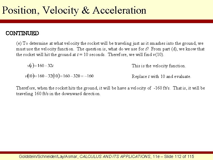
Position, Velocity & Acceleration CONTINUED (e) To determine at what velocity the rocket will be traveling just as it smashes into the ground, we must use the velocity function. The question is, what do we use for t? From part (d), we know that the rocket will hit the ground at t = 10 seconds. Therefore, we will find v(10). This is the velocity function. Replace t with 10 and evaluate. Therefore, when the rocket hits the ground, it will be have a velocity of -160 ft/s. That is, it will be traveling 160 ft/s in the downward direction. Goldstein/Schneider/Lay/Asmar, CALCULUS AND ITS APPLICATIONS, 11 e – Slide 112 of 115

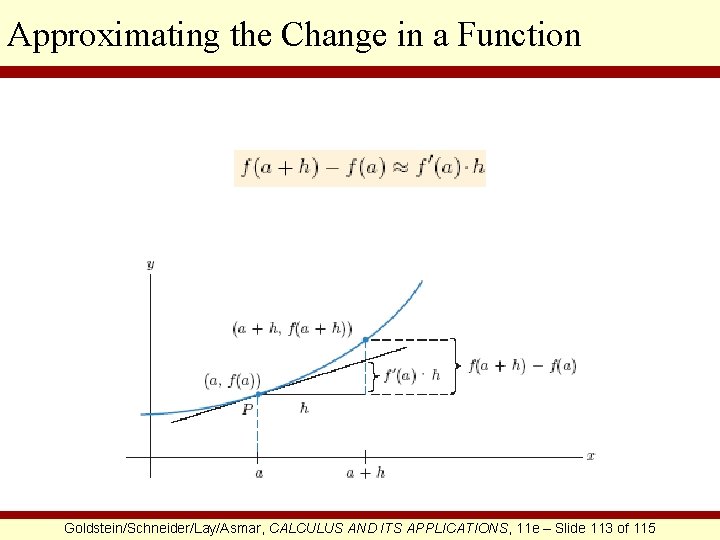
Approximating the Change in a Function Goldstein/Schneider/Lay/Asmar, CALCULUS AND ITS APPLICATIONS, 11 e – Slide 113 of 115

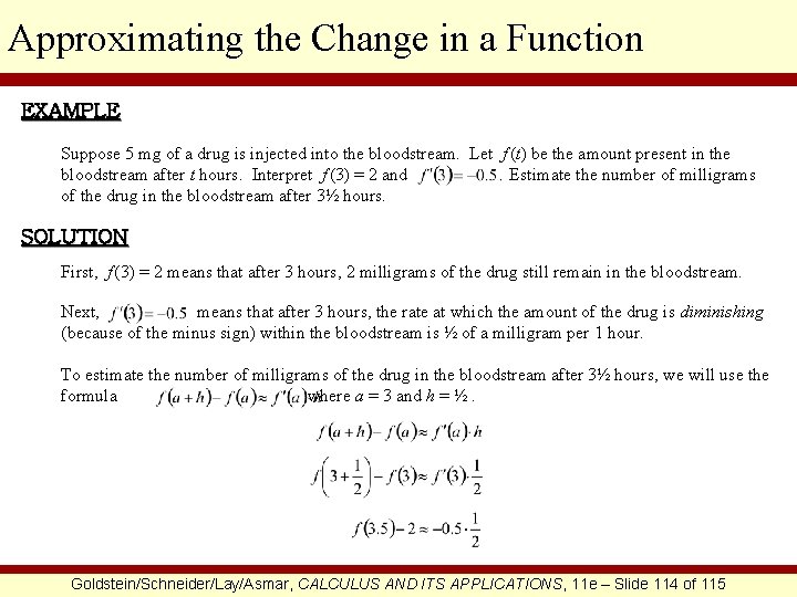
Approximating the Change in a Function EXAMPLE Suppose 5 mg of a drug is injected into the bloodstream. Let f (t) be the amount present in the bloodstream after t hours. Interpret f (3) = 2 and Estimate the number of milligrams of the drug in the bloodstream after 3½ hours. SOLUTION First, f (3) = 2 means that after 3 hours, 2 milligrams of the drug still remain in the bloodstream. Next, means that after 3 hours, the rate at which the amount of the drug is diminishing (because of the minus sign) within the bloodstream is ½ of a milligram per 1 hour. To estimate the number of milligrams of the drug in the bloodstream after 3½ hours, we will use the formula where a = 3 and h = ½. Goldstein/Schneider/Lay/Asmar, CALCULUS AND ITS APPLICATIONS, 11 e – Slide 114 of 115

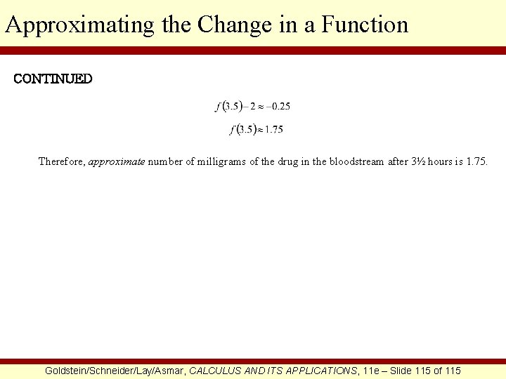
Approximating the Change in a Function CONTINUED Therefore, approximate number of milligrams of the drug in the bloodstream after 3½ hours is 1. 75. Goldstein/Schneider/Lay/Asmar, CALCULUS AND ITS APPLICATIONS, 11 e – Slide 115 of 115